Supervised Learning

What is Supervised Learning? Maybe that’s one of your big questions when you get into this topic. But, before digging deeper into Supervised Learning, it’s a good idea to first do a quick recap about Machine Learning and what it has to do with Supervised Learning.

Introduction to Machine Learning

Machine Learning (ML) is a subset of Artificial Intelligence (AI) that allows software applications to become more accurate in predicting outcomes without being explicitly programmed. In simple terms, it provides machines the ability to automatically learn and improve from experience.

It’s like teaching a small child how to walk. First, the kid observes how others do it, then they try to do it themselves and keep on trying until they walk perfectly. This process involves a lot of falling and getting up. Similarly, in machine learning, models are given data, with which they make predictions. Based on the outcome of those predictions—right or wrong, the models adjust their behaviours, learning and improving over time to make accurate predictions.

According to Arthur Samuel (American pioneer in AI and gaming), Machine Learning is a field of study that gives computers the ability to learn without being explicitly programmed.

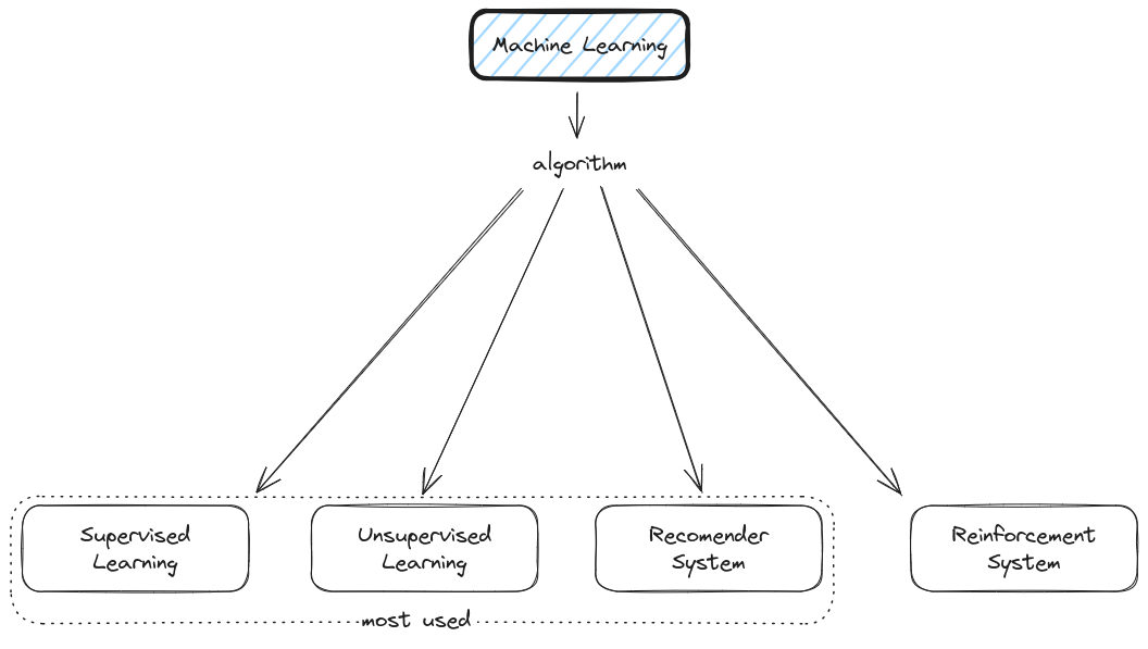
Definition and types of Machine Learning Algorithms

There are various machine learning algorithms:

Supervised Learning - In supervised learning, we provide the machine with labelled input data and a correct output. In other words, we guide the machine towards the right output. It’s kind of like a student learning under the guidance of a teacher. The ‘teacher’, in this case, is the label that tells the model about the data so it can learn from it. Once the model is trained with this labelled data, it can start to make predictions or decisions when new, unlabeled data is fed to it. A common example of supervised learning is classifying emails into “spam” or “not spam”.
Unsupervised Learning - Unlike supervised learning, we do not have the comfort of a ‘teacher’ or labelled data here. In unsupervised learning, we only provide input to the machine learning model but no corresponding output. That is, the model is not told the right answer. The idea is for the model to explore the data and find some structure within. A classic example of unsupervised learning is customer segmentation, where you want to group your customers into different segments based on purchasing behaviour, but you don’t have any pre-existing labels.
Recommender Systems - Imagine walking into a bookstore and having an expert assistant who knows your reading habits guide you to books that would perfectly suit your taste – wouldn’t it be a delight? This is what recommender systems strive to do in virtual environments. They are intelligent algorithms that create a personalized list of suggestions based on data about each user’s past behaviour or user-item interactions.
Reinforcement Learning - This is a bit like learning to ride a bike. You don’t know how to do it at first, but with trial and error, you learn that pedalling keeps you balanced and turning the handlebars allows you to change direction. That’s essentially how reinforcement learning works - the model learns by interacting with its environment and receiving rewards or penalties.

What is Supervised Learning?

Now, let’s dig deeper into supervised learning, as it’s the most commonly used type of machine learning.

In supervised learning, we train the model using ‘labeled’ data. That means our data set includes both the input ($x$) data and its corresponding correct output ($y$). This pair of input-output is also known as a ‘feature’ and a ‘label’. An easy way to think about this is with a recipe: the ‘feature’ is a list of ingredients (our input), and the ‘label’ is the dish that results from those ingredients (our correct output).

The algorithm analyses this input-output pair, maps the function that transforms input to output, and tries to gain understanding of such relationship so that it can apply it to unlabeled, new data.

There are two main types of problems that Supervised Learning tackles: Regression and Classification. 1. Regression: predict a number from many possible numbers (like predicting the price of a house based on its features like size, location etc.). 2. Classification: predicts only a small number of possible outputs or categories (like determining whether an email is spam or not spam, or whether a tumor is malignant or benign, or the picture is of a cat or a dog etc.)

Overall, supervised learning offers an efficient way to use known data to make meaningful predictions about new, future data. By analyzing the relationships within labeled training data, supervised learning models can then apply what they’ve learned to unlabeled, real-world data and make informed decisions or predictions.

Linear Regression

Let’s dive into one of the most basic and fundamental algorithms in the realm of Supervised Learning: Linear Regression.

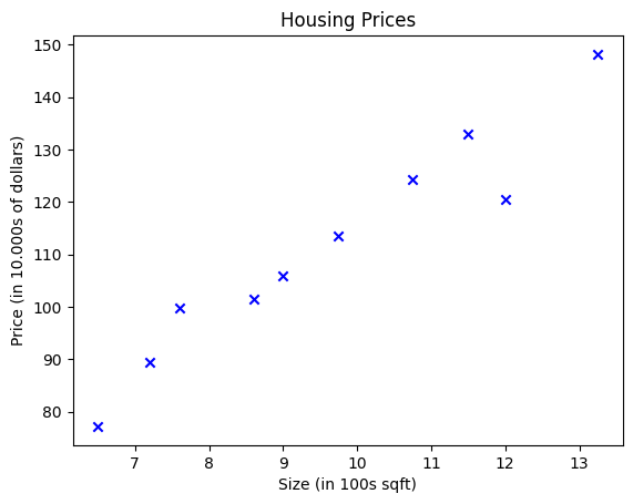
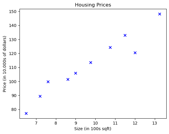
import numpy as np
import matplotlib.pyplot as plt

x_train = np.array([6.50, 7.60, 12.00, 7.20, 9.75, 10.75, 9.00, 11.50, 8.60, 13.25])
y_train = np.array([77.2, 99.8, 120.5, 89.5, 113.5, 124.2, 106.0, 133.0, 101.5, 148.2])

# Plot the data points
plt.scatter(x_train, y_train, marker='x', c='b')
# Set the title
plt.title("Housing Prices")
# Set the y-axis label
plt.ylabel('Price (in 10.000s of dollars)')
# Set the x-axis label
plt.xlabel('Size (in 100s sqft)')
plt.show()

Introduction to Linear Regression

Imagine you’re a real estate agent, and you’re helping customers sell their houses at a reasonable market price. To do this, you need a way to predict a house’s market price based on its characteristics, such as the number of rooms, the year it was built, the neighborhood it’s in, etc.

This is where Linear Regression comes in!

Linear Regression is like drawing a straight line through a cloud of data points. The line represents the relationship between the independent variables (the house characteristics, or ‘features’) and the dependent variable (the house price, or ‘target variable’).

But you might be wondering, “Why is it called ‘Linear’ Regression?” Well, it’s because this approach assumes that the relationship between the independent and dependent variables is linear. This simply means that if you were to plot this relationship on a graph, you could draw a straight line, or ‘linear’ line, to represent this relationship.

In simple terms, we’re trying to draw a line of best fit through our data points that minimizes the distance between the line and all the data points. Let’s take a look below, this is how the linear regression process works:

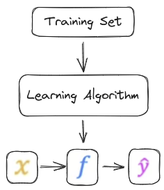
Supervised Learning includes both the input features and also the output targets, The output targets are the right answers to the model we’ll learn from. To train the model, you feed the training set, both the input features and the output targets to your learning algorithm. Then your supervised learning algorithm will produce some function ($f$). The job with $f$ is to take a new input $x$ and output and estimate or a prediction ($\hat{y}$), In machine learning, the convention is that $\hat{y}$ is the estimate or the prediction for $y$.

The model for Linear Regression is a linear function of the input features. It’s represented as:

\[ f(x_{(i)}) = wx_{(i)} + b\]

General Notation	Description
$x$	Training Example feature values
$x_{(i)}$	$i_{th}$Training Example
$\hat{y}$	Training Example targets
m	Number of training examples
$w$	parameter: weight
$b$	parameter: bias
$f$	The model for Linear Regression

If you pay attention, in a linear function there are $w$ and $b$. The $w$ and $b$ are called the parameters of the model. In machine learning parameters of the model are the variables you can adjust during training in order to improve the model. Sometimes you also hear the parameters $w$ and $b$ referred to as weights and bias. Now let’s take a look at what these parameters $w$ and $b$ do.

import numpy as np
import matplotlib.pyplot as plt

x = np.arange(0, 5)
y = np.arange(0, 5)

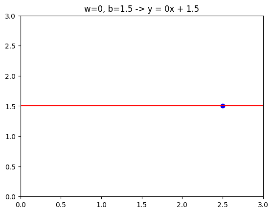
Case 1

If $w$ = 0 and $b$ = 1.5, then $f$ looks like a horizontal line.

In this case the function $f (x)=0 * x + 1.5 $ so $f$ is always constant. It always predicts 1.5 for the estimated $y$ value.

$\hat{y}$ is always equal to $b$ and here $b$ is also called y-intercept because it intersects the vertical axis or y-axis on this graph.

w = 0
b = 1.5

def compute(x, w, b):
    return w * x + b

tmp_fx = compute(x, w, b,)

tmp_x = 2.5
y = w * tmp_x + b

plt.plot(x, tmp_fx, c='r')
plt.scatter(tmp_x, y, marker='o', c='b')
plt.xlim(0, 3)
plt.ylim(0, 3)
plt.title("w=0, b=1.5 -> y = 0x + 1.5")
plt.show()

Case 2

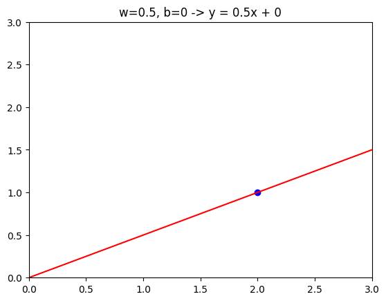
If $w$ = 0.5 and $b$ = 0, then $f(x)=0.5 * x $.

If $x$ = 0 then the prediction is also 0, and if $x$ = 2 then the prediction is 0.5 * 2 which is 1.

You get a line like this and notice that the slope is 0.5 / 1. The value of $w$ gives you the slope of the line , which is 0.5

w = 0.5
b = 0

def compute(x, w, b):
    return w * x + b

tmp_fx = compute(x, w, b,)

tmp_x = 2
y = w * tmp_x + b

plt.plot(x, tmp_fx, c='r')
plt.scatter(tmp_x, y, marker='o', c='b')
plt.xlim(0, 3)
plt.ylim(0, 3)
plt.title("w=0.5, b=0 -> y = 0.5x + 0")
plt.show()

Case 3

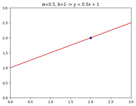
If $w$ = 0.5 and $b$ = 1, then $f(x)=0.5 * x + 1$. and if $x$ = 0, then $f(x)= b$, which is 1. So the line intersects the vertical axis at $b$, the intersection $y$ .

Also if $x$ = 2, then $f(x)= 2$, so the line looks like this.

Again, this slope is 0.5 / 1 so the value of $w$ results in a slope of 0.5.

w = 0.5
b = 1

def compute(x, w, b):
    return w * x + b

tmp_fx = compute(x, w, b,)

tmp_x = 2
y = w * tmp_x + b

plt.plot(x, tmp_fx, c='r')
plt.scatter(tmp_x, y, marker='o', c='b')
plt.xlim(0, 3)
plt.ylim(0, 3)
plt.title("w=0.5, b=1 -> y = 0.5x + 1")
plt.show()

Let’s consider a simple case study by Predicting a house’s price based on its size. The train set can be represented as follows:

House Size (100 sq.ft) ($x$)	Price (10.000s USD) ($y$)
6.5	77.2
7.6	99.8
12.0	120.5
7.20	89.5
9.75	113.5
10.75	124.2
9.0	106.0
11.5	133.0
8.6	101.5
13.25	148.2

Explanation:

In this example, we have house sizes as our independent variable (input) and corresponding house price as the dependent variable (output we want to predict). Assuming a linear relationship between size and price, we can use a linear regression model to predict the price based on the size.

import numpy as np
import matplotlib.pyplot as plt

x_train = np.array([6.50, 7.60, 12.00, 7.20, 9.75, 10.75, 9.00, 11.50, 8.60, 13.25])
y_train = np.array([77.2, 99.8, 120.5, 89.5, 113.5, 124.2, 106.0, 133.0, 101.5, 148.2])

# Plot the data points
plt.scatter(x_train, y_train, marker='x', c='b')
# Set the title
plt.title("Housing Prices")
# Set the y-axis label
plt.ylabel('Price (in 10.000s of dollars)')
# Set the x-axis label
plt.xlabel('Size (in 100s sqft)')
plt.show()

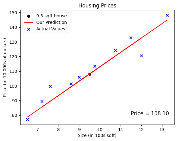
Now, the question is: How to predict the price of 9.5 sqft house? We can use the Linear Regression model to predict this.

With the amount of data we have, it would be difficult if we did 1 by 1 calculations manually. So, you can compute the function output in a for loop as shown in the compute_output function below.

def compute_output(x, w, b):
    """
    Computes the prediction of a linear model
    Args:
      x    : Data, m examples 
      w,b  : model parameters  
    Returns
      f_wb : model prediction
    """
    m = len(x_train)
    f_wb = w * x + b

    return f_wb

# Please replace the values of w and b with numbers that you think are appropriate
w = 9.8
b = 15

tmp_f_wb = compute_output(x_train, w, b,)

# predict the price of 9.5 sqft house
tmp_x = 9.5
y_hat = w * tmp_x + b

# Plot the price of 9.5 sqft house
plt.scatter(tmp_x, y_hat, marker='o', c='black',label='9.5 sqft house')
plt.text(11.5, 80, f"Price = {y_hat:.2f}", fontsize=12)

# Plot our model prediction
plt.plot(x_train, tmp_f_wb, c='r',label='Our Prediction')

# Plot the data points
plt.scatter(x_train, y_train, marker='x', c='b',label='Actual Values')

# Set the title
plt.title("Housing Prices")
# Set the y-axis label
plt.ylabel('Price (in 10.000s of dollars)')
# Set the x-axis label
plt.xlabel('Size (in 100s sqft)')
plt.legend()
plt.show()

Loss function

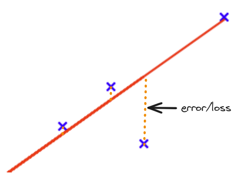
Now, how do we know if the line is a good fit?

We can calculate the error between the predicted value and the actual value.

For example, if the actual value is $y$, and the predicted value is $\hat{y}$, then the error is $y - \hat{y}$.

We can calculate the error for each data point, and then sum them up.

The error function is:

\[ E = \sum_{i=1}^{n} (y_i - \hat{y_i})^2 \]

where $y$ is the actual value, and $\hat{y}$ is the predicted value.

This is called the sum of squared errors. (SSE)

import numpy as np
import matplotlib.pyplot as plt
import ipywidgets as widgets
from IPython.display import display

x_data = np.random.rand(100) * 10
noise = np.random.normal(0, 2, x_data.shape)
y_data = 3*x_data + 8 + noise

# Define the update function
def update(a, b):
    y = a*x + b
    plt.plot(x, y, color='red')
    plt.scatter(x_data, y_data, s=1)
    plt.xlabel('x')
    plt.ylabel('y')

    plt.title(f"Equation y = {a}x + {b}")

    # Calculate the loss
    loss = np.sum((y_data - y)**2)

    # Draw the loss
    plt.text(0, 20, f"Loss = {loss:.2f}", fontsize=12)

    plt.show()

# Create scattered dot around y = 3x + 8
x = np.random.rand(100) * 10
noise = np.random.normal(0, 2, x.shape)
y = 3*x + 8 + noise

# Define the slider widgets
a_slider = widgets.FloatSlider(min=0, max=10, step=0.1, value=0, description='a:')
b_slider = widgets.FloatSlider(min=0, max=10, step=0.1, value=0, description='b:')

# Display the widgets and plot
widgets.interactive(update, a=a_slider, b=b_slider)

So, the goal of linear regression is to find the best a and b that minimize the loss function.

In other words, we want to find the best a and b that make the red line as close as possible to the scattered dots.

Other Loss Functions

There are other loss functions, for example:

Mean Square Error (MSE)

\[ E = \frac{1}{n} \sum_{i=1}^{n} (y_i - \hat{y_i})^2 \]

Mean Absolute Error (MAE)

\[ E = \sum_{i=1}^{n} |y_i - \hat{y_i}| \]

Root Mean Squared Error (RMSE)

\[ E = \sqrt{\frac{1}{n}\sum_{i=1}^{n} (y_i - \hat{y_i})^2} \]

RMSE is in the same units as the target variable, which can make it more interpretable in some cases.

The loss function, also called the cost function, tells us how well the model performs so we can try to make it better. The cost function itself measures the difference (error/loss rate) between the model prediction and the actual value for $y$.

Let’s break down the formula for SSE to help you understand:

The cost function takes the prediction y hat and compares it to the target $y$ by taking $\hat{y}$ minus $y$

\[ (f(x^{(i)}) - y^{(i)})^2 \]

Then, the formula is the sum of the absolute value of the diff

\[J(w,b) = \sum\limits_{i = 0}^{m-1} (f(x^{(i)}) - y^{(i)})^2\]

But that equation is not fair because it doesn’t take into account the number of examples we have. So we divide it by the number of examples, $m$.

\[J(w,b) = \frac{1}{m} \sum\limits_{i = 0}^{m-1} (f(x^{(i)}) - y^{(i)})^2\]

where \[f(x^{(i)}) = wx^{(i)} + b\]

$f(x^{(i)})$ is our prediction for example $i$ using parameters $w,b$.
$(f(x^{(i)}) -y^{(i)})^2$ is the squared difference between the target value and the prediction.
These differences are summed over all the $m$ examples and divided by m to produce the cost, $J(w,b)$.

Look at the code below, where it will calculate the cost by looping each example. In each loop:

$fx$, a prediction is calculated
the difference between the target and the prediction is calculated and squared.
this is added to the total cost.

def compute_cost(x, y, w, b):
    """
    Computes the cost function for linear regression.

    Args:
      x : Data, m examples
      y : target values
      w,b : model parameters

    Returns
        total_cost (float): The cost of using w,b as the parameters for linear regression
               to fit the data points in x and y
    """
    # number of training examples
    m = len(x_train)

    cost_sum = 0
    for i in range(m):
        fx = w * x[i] + b
        cost = (fx - y[i]) ** 2
        cost_sum = cost_sum + cost
    total_cost = (1 / m) * cost_sum

    return total_cost

x_train = np.array([6.50, 7.60, 12.00, 7.20, 9.75, 10.75, 9.00, 11.50, 8.60, 13.25])
y_train = np.array([77.2, 99.8, 120.5, 89.5, 113.5, 124.2, 106.0, 133.0, 101.5, 148.2])
w = 10
b = 15

errors = compute_cost(x_train, y_train, w, b)
errors
# print(f"Number of errors: {errors}")

Based on the data owned and the value of $w$ and $b$, when viewed from the results of the compute_cost function, the total mistakes we got were 31.641.

Then, is the best amount? Remember that the purpose of linear regression is to minimize total errors.

Then how do you do it? In other words we want to get the best $w$ and $b$ values that make the lines as close as possible to the spread points.

One way is you can use the Scikit-learn library.

import numpy as np

answer = ()
minimum_cost = 100000

for w in np.arange(8.0, 12.0, 0.001):
    for b in np.arange(13.0, 15.0, 0.001):
        cost = compute_cost(x_train, y_train, w, b)
        if cost < minimum_cost:
            minimum_cost = cost
            answer = (w, b)

print(f"Minimum cost: {minimum_cost}")
print(f"w: {answer[0]} b: {answer[1]}")

Scikit-learn for Linear Regression

The sklearn (or Scikit-learn) library in Python is a powerful, open-source library that provides simple and efficient tools for data analysis and modeling, including machine learning. It has numerous features, ranging from simple regression models to complex machine learning models.

For our Linear Regression model, sklearn provides the LinearRegression class within the sklearn.linear_model module.

Here’s how you can do it:

from sklearn.linear_model import LinearRegression

# Reshape the input array
x_train = np.array([6.50, 7.60, 12.00, 7.20, 9.75, 10.75, 9.00, 11.50, 8.60, 13.25]).reshape((-1, 1))
y_train = np.array([77.2, 99.8, 120.5, 89.5, 113.5, 124.2, 106.0, 133.0, 101.5, 148.2])

model = LinearRegression()

# Use this score function to in model.fit
model.fit(x_train, y_train)

# Generates and displays coefficients and intercepts
coefficient = model.coef_ # w
intercept = model.intercept_ # b
print(f"Coefficients: {coefficient}")
print(f"Intercept: {intercept}")

Coefficients: [9.09553728]
Intercept: 23.886409100809274

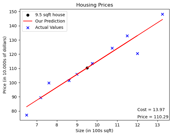
From the results of the code above, the $w$ (coefficient) value is 9.09553728 and $b$ (intercept) is 23.886409100809274. That way we can produce the minimum possible error/loss value. Now we look again at the data we have with the new $w$ and $b$ values and what error/loss we get.

x_train = np.array([6.50, 7.60, 12.00, 7.20, 9.75, 10.75, 9.00, 11.50, 8.60, 13.25])
y_train = np.array([77.2, 99.8, 120.5, 89.5, 113.5, 124.2, 106.0, 133.0, 101.5, 148.2])
w = coefficient[0]
b = intercept

cost = compute_cost(x_train, y_train, w, b)
tmp_f_wb = compute_output(x_train, w, b,)

# predict the price of 9.5 sqft house
tmp_x = 9.5
y_hat = w * tmp_x + b

# Plot the price of 9.5 sqft house
plt.scatter(tmp_x, y_hat, marker='o', c='black',label='9.5 sqft house')
plt.text(12, 75, f"Price = {y_hat:.2f}", fontsize=10)

# Plot our model prediction
plt.plot(x_train, tmp_f_wb, c='r',label='Our Prediction')

# Plot the data points
plt.scatter(x_train, y_train, marker='x', c='b',label='Actual Values')
plt.text(12, 80, f"Cost = {cost:.2f}", fontsize=10)

# Set the title
plt.title("Housing Prices")
# Set the y-axis label
plt.ylabel('Price (in 10.000s of dollars)')
# Set the x-axis label
plt.xlabel('Size (in 100s sqft)')
plt.legend()
plt.show()

Based on the results in the graph above, we can see a decrease in the error/loss that we got, from the previous amount of 31.641 to 27.94. In this way, the level of accuracy in predicting the price of the house we are looking for will increase.

You can also make predictions with this trained model. For example, if you want to predict the y value for x = 9.5, you can do it using the predict() method like this:

x_new = np.array([9.5]).reshape((-1, 1))
y_pred = model.predict(x_new)
print(f"Predicted value for x = 9.5: {y_pred}")

Predicted value for x = 9.5: [110.29401321]

But, how does the sklearn library calculate the best $w$ and $b$ values? The answer is using the Gradient Descent algorithm, which will be discussed in the next section.

Linear Regression with Multiple Input Variables

Multiple Features

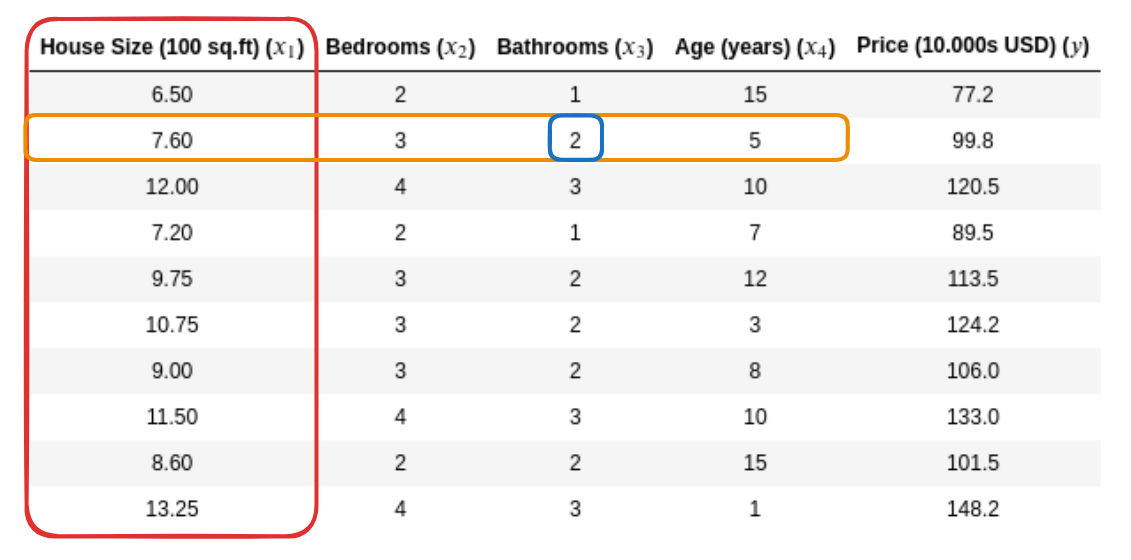
In real-world scenarios, an output variable or a result often depends on more than one factor or input variable. In machine learning, these factors are referred to as “features”. In the previous discussion, you have one feature $x$, the size of the house and you can predict $y$, the price of the house. But now, what if you don’t just use the size of the house as a feature that can be used to predict prices such as the number of bedrooms and bathrooms and the age of the house. Let’s look at the example below:

General Notation	Description
$x_1$	House Size
$x_2$	Number of Bedrooms
$x_3$	Number of Bathrooms
$x_4$	House Age
$y$	Price
$x_{j}$	$j$ Feature (red rectangle)
$n$	Number of Feature
$\vec{x}^{(i)}$	Feature of $i^{th}$ training example, also called a row vector (yellow rectangle)
${\vec{x}_{j}}^{(i)}$	Value of Feature $j$ in $i^{th}$ in the training example (blue rectangle)

If you just used the size of a house to predict its price, it would be a simple linear regression problem. In the previous discussion, this is how we defined the model, with $x$ as a single feature:

\[ f(x) = wx + b\]

But now with many features, we will define them differently. We still multiply $w$ with $x$, but since now we have multiples of $w.x$, we sum them up together. The model then look like this:

\[ f(\vec{x}) = w_{1}x_{1} + w_{2}x_{2} + \dots + w_{n}x_{n} + b\]

or in vector notation can be written like this:

\[ f(\vec{x}) = \vec{w} \cdot \vec{x} + b\]

where $\cdot$ is a vector dot product

General Notation	Description
$\vec{w}$	[ $w_{1}, w_{2}, \dots , w_{n}$ ]
$b$	Number of Bias Parameter
$\vec{x}$	[ $x_{1}, x_{2}, \dots , x_{n}$ ]

Here, $\vec{w}$ are parameters of the model that it learns during the training phase. The $\vec{x}$ are the features. Using multiple features usually gives a better prediction than using just one feature, as real-world scenarios are often influenced by more than just one factor. It’s worth noting, however, that adding more and more features can also lead to overfitting where the model learns the training data too well and performs poorly on unseen data.

Note: We’ll learn more about dot product in the next material on Matrix and Vector.

Let’s go back to our case, where now we have multiple features to predict house prices

House Size (100 sq.ft) ($x_1$)	Bedrooms ($x_2$)	Bathrooms ($x_3$)	Age (years) ($x_4$)	Price (10.000s USD) ($y$)
6.50	2	1	15	77.2
7.60	3	2	5	99.8
12.00	4	3	10	120.5
7.20	2	1	7	89.5
9.75	3	2	12	113.5
10.75	3	2	3	124.2
9.00	3	2	8	106.0
11.50	4	3	10	133.0
8.60	2	2	15	101.5
13.25	4	3	1	148.2

In this example, we not only have the size of the house as the independent variable, but also the number of bedrooms and bathrooms as well as the age of the house itself and don’t forget the price of the house as the dependent variable.

Let’s take what we learn and apply it to code:

X_train = np.array([
    [6.50, 2, 1, 15],
    [7.60, 3, 2, 5],
    [12.00, 4, 3, 10],
    [7.20, 2, 1, 7],
    [9.75, 3, 2, 12],
    [10.75, 3, 2, 3],
    [9.00, 3, 2, 8],
    [11.50, 4, 3, 10],
    [8.60, 2, 2, 15],
    [13.25, 4, 3, 1]
])

y_train = np.array([77.2, 99.8, 120.5, 89.5, 113.5, 124.2, 106.0, 133.0, 101.5, 148.2])

print(f"X Shape: {X_train.shape}, X Type:{type(X_train)})")
print(X_train)
print(f"y Shape: {y_train.shape}, y Type:{type(y_train)})")
print(y_train)

X Shape: (10, 4), X Type:<class 'numpy.ndarray'>)
[[ 6.5   2.    1.   15.  ]
 [ 7.6   3.    2.    5.  ]
 [12.    4.    3.   10.  ]
 [ 7.2   2.    1.    7.  ]
 [ 9.75  3.    2.   12.  ]
 [10.75  3.    2.    3.  ]
 [ 9.    3.    2.    8.  ]
 [11.5   4.    3.   10.  ]
 [ 8.6   2.    2.   15.  ]
 [13.25  4.    3.    1.  ]]
y Shape: (10,), y Type:<class 'numpy.ndarray'>)
[ 77.2  99.8 120.5  89.5 113.5 124.2 106.  133.  101.5 148.2]

For parameter vector $w$ and $b$ can be written like this:

$w$ is a vector with $n$ elements.
- Each element contains the parameter associated with one feature.
- in our dataset, n is 4.
- notionally, we draw this as a column vector
$b$ is a scalar parameter.

b_init = 46.68178303822603
w_init = np.array([ 7.05979876, -4.1870478, 8.30627675, -0.94230069])
print(f"w_init shape: {w_init.shape}, b_init type: {type(b_init)}")

w_init shape: (4,), b_init type: <class 'float'>

Now, let’s look at a basic implementation using a for loop for computing the model’s prediction.

\[f(\vec{x}) = \sum\limits_{j = 1}^{n} w_{j}x_{j} + b\]

def predict_single_loop(x, w, b): 
    """
    single predict using linear regression
    
    Args:
      x (ndarray): Shape (n,) example with multiple features
      w (ndarray): Shape (n,) model parameters    
      b (scalar):  model parameter     
      
    Returns:
      f (scalar):  prediction
    """
    n = len(x)
    f = 0
    for i in range(n):
        f_i = x[i] * w[i]  
        f = f + f_i         
    f = f + b                
    return f

# get a row from our training data
x_vec = X_train[0,:]
print(f"x_vec shape {x_vec.shape}, x_vec value: {x_vec}")

# make a prediction
f_x = predict_single_loop(x_vec, w_init, b_init)
print(f"f_wb shape {f_x.shape}, prediction: {f_x}")

x_vec shape (4,), x_vec value: [ 6.5  2.   1.  15. ]
4
f_wb shape (), prediction: 78.36814577822602

def compute_cost_for_multiple_variables(X, y, w, b):
    """
    Computes the cost function for linear regression.

    Args:
      X : Data, m examples
      y : target values
      w,b : model parameters

    Returns
        total_cost (float): The cost of using w,b as the parameters for linear regression
               to fit the data points in X and y
    """
    m = len(y)  # number of training examples
    
    # hypothesis calculation - output prediction
    fx = np.dot(X, w) + b
    
    # error calculation
    errors = fx - y
    
    # calculate total cost
    total_cost = (1 / m) * np.dot(errors.T, errors)

    return total_cost

Now, there is a very interesting trick called vectorization, which will make it easier to implement this algorithm and many other learning algorithms. And it will runs much faster too! Let’s go into the next discussion to see what vectorization is.

Vectorization

Vectorization is a powerful ability within NumPy (and other similar libraries) to express operations as occurring on entire arrays, rather than their individual elements.

When we loop over elements of an array and perform operations, this is called scalar computation. In Python, scalar computation is relatively slow compared to vectorized computation. This is where vectorization can be of great use in machine learning tasks which often require performing operations on large amounts of data.

Now, let’s look at how we can do this using vectorization.

\[ f(\vec{x}) = \vec{w} \cdot \vec{x} + b\]

And now you can implement it with one line of code like below using dot() method from NumPy:

def predict(x, w, b): 
    """
    single predict using linear regression
    
    Args:
      x (ndarray): Shape (n,) example with multiple features
      w (ndarray): Shape (n,) model parameters   
      b (scalar):             model parameter 
      
    Returns:
      f (scalar):  prediction
    """
    f = np.dot(x, w) + b     
    return f

# get a row from our training data
x_vec = X_train[0,:]
print(f"x_vec shape {x_vec.shape}, x_vec value: {x_vec}")

# make a prediction
f_wb = predict(x_vec,w_init, b_init)
print(f"f_wb shape {f_wb.shape}, prediction: {f_wb}")

x_vec shape (4,), x_vec value: [ 6.5  2.   1.  15. ]
f_wb shape (), prediction: 78.36814577822602

How many features do we need?

In the previous discussion, we have discussed how to use multiple features to predict house prices. But, how many features do we need?

Should we add the following features to our model? - The number of floors - The size of the backyard - Is it near a school? - Is it near a mall? - Does it have a swimming pool?

More features are not always better. Adding more features can lead to overfitting, where the model learns the training data too well and performs poorly on unseen data.

Feature Engineering

Feature choices can have a big impact on the performance of your learning algorithm. In fact, for many practical applications, selecting or including the right features is a critical step for an algorithm to function properly. In this topic, let’s see how we can select or engineer the most suitable features for our learning algorthm.

Feature Engineering is the process of transforming raw data into features that better represent the underlying problem to the predictive models, resulting in improved model accuracy on unseen data. In other words, you’re creating new features from the existing ones, or even removing some that you deem unnecessary.

Feature engineering can be considered as adding more useful information for your model to learn from. In the context of linear regression with multiple input variables, feature engineering can be crucial because the relationship between the response variable and predictors may not always be linear or may depend on multiple interacting variables.

For a dataset describing different lands, let’s say we have three original features – Width, Depth, and Price:

LandID	Width (m)	Depth (m)	Price ($)
1	10	20	2000
2	20	15	3000
3	15	20	2500
4	10	12	1200
5	12	15	2250

The simple Machine learning model using Width and Depth to predict price could look like this:

\[ f(\vec{x}) = w_{1}x_{1} + w_{2}x_{2} + b\]

Now let’s see how feature engineering can enhance this dataset.

Creating new features

One simple feature engineering task on this dataset could be creating a new feature representing the total area. While the width and depth by themselves might not be the best indicators of price, land area (calculated as depth x width) could be a stronger feature.

LandID	Width (m)	Depth (m)	Area (m²)	Price ($)
1	10	20	200	2000
2	20	15	300	3000
3	15	20	300	2500
4	10	12	120	1200
5	12	15	180	2250

In certain situations, raw features as given in the dataset might not have a clear and direct relationship with the target variable. In the example of predicting land price, it’s possible that neither the depth nor the width of the land independently has a strong predictable effect on the price.

However, when you combine them into a single feature (the total area, which is depth multiplied by width), you can create a new representation of your data that might have a better correlation or association with the target variable (price, in this case). It’s common that a property, such as area here, can have more correlation to price than either width or depth individually.

In other words, even though the width and depth independently may not be good predictors, their product (which represents the total area) might prove to be a very good predictor. This can be understood intuitively too - larger lands (greater area) usually cost more.

This process of creating new and more effective features is a key part of feature engineering. Good feature engineering can often make the difference between a weak model and a highly accurate one. It’s an essential step in any machine learning project and often requires knowledge about the domain from which the data originates

Now with the new feature, the Machine Learning model will look like this:

\[ f(\vec{x}) = w_{1}x_{1} + w_{2}x_{2} + w_{3}x_{3} + b\]

Why Feature Engineering important in Linear Regression

Linear regression aims to establish a linear relationship between the input variables (features) and the single output variable (target). Feature engineering aids in improving this relationship, leading to more accurate models. Good features capture important aspects of the data and provide information that helps the model make correct predictions.

When it comes to linear regression, the importance of feature engineering arises from the fact that the model is quite simple. The model assumes a simple linear relationship between input and outputs. If the features can capture complex dependencies in simple forms, the model has a much easier time learning from them.

It is also important to note that feature engineering often requires domain knowledge. In the land-price example, knowing that land price is often a function of total area is key to creating the “area” feature from the original “width” and “depth” features. As such, while Machine Learning provides many powerful tools, domain expertise is often key to applying these tools effectively.

Here are some common methods used in feature engineering:

Feature scaling: This includes methods such as standardization and normalization. Feature scaling is used to standardize the range of features of data. This is important because features might have different units and may vary in range. Some algorithms, like gradient descent, converge faster when features are on a similar scale.
Polynomial features: This is useful when the relationship between the independent and dependent variable is not linear. Polynomial features create interactions between features and also create features to the power of the exponent. For example, if we have a feature $x$, we can create a new feature that is $x^2$ or $x^3$.

Feature Scalling

Feature Scalling is a technique that will enable gradient descent (the algorithm behind model.fit) to run much faster. Feature scaling is a step in data preprocessing that aims to standardize the range of features in the data. When the range of values in different features varies greatly, the ML algorithm might take longer to converge, or it may not effectively learn the correct weights for each feature.

Two common types of feature scaling are: - Mean Normalization - Standardization (Z-score Scaling)

Notes: To find out what gradient descent is, it will be discussed in the next material.

Mean Normalization

This method centers the data around 0. It scales the data between -1 and 1 by subtracting each observation by the average of observations and then dividing by the difference between the maximum and minimum value.

\[x_i := \dfrac{x_i - \mu_i}{max - min} \]

So, when do we use it? Mean Normalization is used when we want to center our variables around zero and vary between -1 and 1. Mean normalization can be useful in cases where we want to eliminate the effect of the units on an algorithm. It’s particularly good when our data has outliers, as mean normalization does not bound values to a specific range.

Below is a Python example to illustrate this:

import numpy as np

# Here is an array with some numbers
x = np.array([
    [650, 2, 1, 15],
    [760, 3, 2, 5],
    [1200, 4, 3, 10],
    [720, 2, 1, 7],
    [975, 3, 2, 12],
    [1075, 3, 2, 3],
    [900, 3, 2, 8],
    [1150, 4, 3, 10],
    [860, 2, 2, 15],
    [1325, 4, 3, 1]
], dtype=float)

# Mean normalization
x_mean_norm = (x - np.mean(x)) / (np.max(x) - np.min(x))
print('Mean Normalized data:')
print(x_mean_norm)

Mean Normalized data:
[[ 0.18518519 -0.48148148  0.51851852]
 [ 0.51851852 -0.14814815 -0.14814815]
 [-0.14814815  0.18518519 -0.48148148]]

Standardization (Z-score Scaling)

This method transform the feature to have a mean of 0 and standard deviation of 1 by subtracting each value by the mean and then dividing by the standard deviation.

Why do we use standardization? If a feature in our dataset has a variance that is orders of magnitude larger than others, it might dominate the objective function and make the estimator unable to learn from other features correctly, leading to sub-optimal performance. Standardization mitigates this issue.

To implement z-score normalization, adjust our input values as shown in this formula: \[x^{(i)}_j = \dfrac{x^{(i)}_j - \mu_j}{\sigma_j}\] where $j$ selects a feature or a column in the $\mathbf{X}$ matrix. $µ_j$ is the mean of all the values for feature (j) and $\sigma_j$ is the standard deviation of feature (j). \[ \begin{align} \mu_j &= \frac{1}{m} \sum_{i=0}^{m-1} x^{(i)}_j\\ \sigma^2_j &= \frac{1}{m} \sum_{i=0}^{m-1} (x^{(i)}_j - \mu_j)^2 \end{align} \]

Here’s an illustrative Python example using sklearn library’s StandardScaler:

from sklearn.preprocessing import StandardScaler
import numpy as np

# Here is an array with some random numbers
x = np.array([
    [650, 2, 1, 15],
    [760, 3, 2, 5],
    [1200, 4, 3, 10],
    [720, 2, 1, 7],
    [975, 3, 2, 12],
    [1075, 3, 2, 3],
    [900, 3, 2, 8],
    [1150, 4, 3, 10],
    [860, 2, 2, 15],
    [1325, 4, 3, 1]
], dtype=float)

# Standardization
std_scaler = StandardScaler()
x_std = std_scaler.fit_transform(x)

print('Standardized data:')
print(x_std)

Standardized data:
[[ 0.         -1.22474487  1.33630621]
 [ 1.22474487  0.         -0.26726124]
 [-1.22474487  1.22474487 -1.06904497]]

The output dimensions of standardization do not have a particular range, which means the data can be negative, zero, or positive. This kind of scaling is less affected by outliers or extreme values as it is based on the mean and standard deviation.

Rule of Thumb Feature Scaling

Feature Range	Status
0 $ x_1 $ 3	ok, no rescaling
-2 $ x_2 $ 0.5	ok, no rescaling
-100 $ x_3 $ 100	too large, rescaling
-0.001 $ x_4 $ 0.001	too small, rescaling

Polynomial Regression

Now, we have learned that linear regression algorithm can find a linear line that best fits the data. But, what if the data is not linear? What if the data is curved?

Polynomial Regression is a form of regression analysis in which the relationship between the independent variable $x$ and the dependent variable $y$ is modeled as an nth degree polynomial. Polynomial regression fits a nonlinear relationship between the value of $x$ and the corresponding conditional mean of $y$.

For example, a simple linear regression equation represent like this: \[ f(x) = wx + b\]

However, in polynomial regression, you might have an equation that looks like this for a second degree (quadratic) polynomial:

\[f(x)= w_0{x_0}^2 + b\]

This equation is still linear in the coefficients. The linearity in polynomial regression applies to the coefficients, and not the degree of the variables.

Polynomial regression can be very useful. When a linear regression model is not sufficient to capture the data relationships, it can be extended with polynomial features.

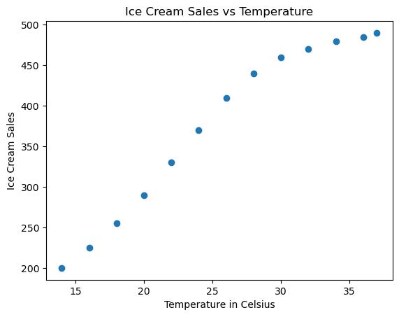
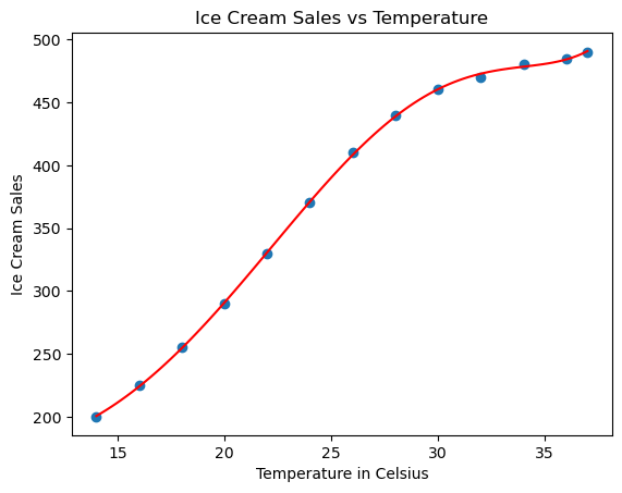
Let’s consider a simple case study. Imagine we are running a small business selling ice cream. We notice that the sales of our ice cream seems to be heavily influenced by the temperature outside.

Let’s say we’ve collected the following data regarding outside temperature (in Celsius) and ice cream sales for a few days:

Temperature (In Celsius) ($x$)	Ice Cream Sales ($y$)
14	200
16	225
18	255
20	290
22	330
24	370
26	410
28	440
30	460
32	470
34	480
36	485
37	490

import numpy as np

x_train = np.array([14, 16, 18, 20, 22, 24, 26, 28, 30, 32, 34, 36, 37])
y_train = np.array([200, 225, 255, 290, 330, 370, 410, 440, 460, 470, 480, 485, 490])

We’re going to visualize our data first to get a better understanding

import matplotlib.pyplot as plt

plt.scatter(x_train, y_train)
plt.xlabel('Temperature in Celsius')
plt.ylabel('Ice Cream Sales')
plt.title('Ice Cream Sales vs Temperature')
plt.show()

Our data appears to show a non-linear trend (increases, then decreases). So, we decided to use quadratic Polynomial Regression to model this data. In this case we will use the sklearn library. sklearn itself provides the PolynomialFeatures class in the sklearn.preprocessing module.

The PolynomialFeatures class in the sklearn.preprocessing module is a feature transformation tool in Scikit-learn. It generates a new matrix consisting of all polynomial combinations of the features with degree less than or equal to the specified degree.

If we have one feature (x), PolynomialFeatures would transform this based on the degree parameter. For a degree of 2, it would transform it to [1, x, x^2]. For a degree of 3, it would transform it to [1, x, x^2, x^3] and so on. The 1 is included as it acts as the intercept term.

Here’s an example of how to use PolynomialFeatures:

from sklearn.preprocessing import PolynomialFeatures
import numpy as np

# Given a simple 2D numpy array
X = np.arange(6).reshape(3, 2)
print("Original Data:")
print(X)

# Create a PolynomialFeatures object and transform the data
poly = PolynomialFeatures(2) # let's choose degree 2
X_poly = poly.fit_transform(X)

print("Transformed Data:")
print(X_poly)

Now, we return to our case example.

from sklearn.preprocessing import PolynomialFeatures
from sklearn.linear_model import LinearRegression

# Transform our x input to 1D array for fitting
x_train_fit = x_train.reshape(-1, 1)

# Create Polynomial Features
poly = PolynomialFeatures(degree=[2, 6])
x_poly = poly.fit_transform(x_train_fit)

# Fit the Polynomial Features to the Linear Regression
poly_model = LinearRegression()
poly_model.fit(x_poly, y_train)

# Generate a sequence of temperatures for prediction 
num_samples = 100
X_seq = np.linspace(x_train_fit.min(),x_train_fit.max(),num_samples).reshape(-1,1)

# Use model to predict ice cream sales
y_poly_pred = poly_model.predict(poly.fit_transform(X_seq))

# Visualize the original data and the polynomial fit
plt.scatter(x_train, y_train)
plt.plot(X_seq, y_poly_pred, color='r')
plt.xlabel('Temperature in Celsius')
plt.ylabel('Ice Cream Sales')
plt.title('Ice Cream Sales vs Temperature')
plt.show()

Now we have a model that not only fits our training data but can predict the ice cream sales at any given temperature, which will help in managing our ice cream supply based on predicted sales.

General Notation	Description
\(x_1\)	House Size
\(x_2\)	Number of Bedrooms
\(x_3\)	Number of Bathrooms
\(x_4\)	House Age
\(y\)	Price
\(x_{j}\)	\(j\) Feature (red rectangle)
\(n\)	Number of Feature
\(\vec{x}^{(i)}\)	Feature of \(i^{th}\) training example, also called a row vector (yellow rectangle)
\({\vec{x}_{j}}^{(i)}\)	Value of Feature \(j\) in \(i^{th}\) in the training example (blue rectangle)

General Notation	Description
\(\vec{w}\)	[ \(w_{1}, w_{2}, \dots , w_{n}\) ]
\(b\)	Number of Bias Parameter
\(\vec{x}\)	[ \(x_{1}, x_{2}, \dots , x_{n}\) ]