!pip install rggraderVisualizing linear algebra as vector spaces
Learning matrices, dot product, linear transformation, or anything that is related to linear algebra can be a bit abstract and can be daunting. One of the best ways to understand linear algebra is to visualize it because surprisingly, linear algebra can be a lot easier to understand when you can see it.
Vector
There should be a video above, if it does not load, click this link: Single Vector Scene
A single vector is a single data point that has multiple dimensions and placed in a dimensional space, which a single dimension represents a single feature. A feature is a single property of a data point.
For example, if we have a data point of a person’s height and weight, we can represent it as a vector of 2 dimensions, where the first dimension is the height (which we can represent as x axis) and the second dimension is the weight (which we can represent as y axis). Each dimension is a feature of the data point.
Here is an example for a vector of 3 dimensions (plotted at x = 2, y = 2, z = 2):

Matrix
In linear algebra a dataset is represented as a matrix. A matrix is a collection of vectors. Every column in a matrix is a vector and every row is a property of the data, it’s commonly called a feature.
\(\begin{bmatrix} x \\ y \\ z \end{bmatrix}\)
Above is a single data point of 3 dimensions or 3 features.
\(\begin{bmatrix} x_0 & x_1 & \ldots & x_n \\ y_0 & y_1 & \ldots & y_n \\ z_0 & z_1 & \ldots & z_n \end{bmatrix}\)
Above matrix we have 3 dimensions or 3 features, and n data points. For example if we have data for student’s evaluation result, every dimension can be the student’s score for each subject (for example math for x, physics for y, and chemistry for z), and every row is a student.
The concept when we’re grouping several vectors into a matrix, it’s called an augmented matrix.
No curves
In linear algebra, we don’t have curves. The vectors will always be straight. Unlike in calculus where we have curves if we’re working with polynomial functions.
The manipulation of space: Essence of linear algebra
Below we have 2 x 1 matrix (2 rows and 1 column) which is a vector of 2 dimensions.
$ \[\begin{bmatrix} x \\ y \end {bmatrix}\] \[\begin{bmatrix} 2 \\ 1 \end{bmatrix}\]$
Of course you should’ve already been familiar with matrix multiplication like below formula
\(\begin{bmatrix} 0 & -1 \\ 1 & 0 \end{bmatrix} \begin{bmatrix} 2 \\ 1 \end{bmatrix} = \begin{bmatrix} -1 \\ 2 \end{bmatrix}\)
But do you know we can visualize above “tranformation” to a “space manipulation” like below?
There should be a video above, if it does not load, click this link: Matrix Multiplication Scene
As you can see, our \(\begin{bmatrix} 2 \\ 1 \end{bmatrix}\) is transformed to \(\begin{bmatrix} -1 \\ 2 \end{bmatrix}\) matrix
This \(\begin{bmatrix} 0 & -1 \\ 1 & 0 \end{bmatrix}\) matrix is also known as rotation matrix, and for this matrix it will rotate the vector 90 degrees counter-clockwise.
Augmented matrix
So if we have lots of data points, we can transform all of them using this very same matrix. For example if we have 6 data points, we can represent them as a matrix of 2 x 6 (2 rows and 6 columns) like below
\[\begin{bmatrix} 0 & -1 \\ 1 & 0 \end{bmatrix} \begin{bmatrix} 2 & 3 & -3 & -2 & 4 & 2 \\ 1 & 3 & 1 & -3 & -3 & 0 \end{bmatrix} = \begin{bmatrix} -1 & -3 & -1 & 3 & 3 & 0 \\ 2 & 3 & -3 & -2 & 4 & 2 \end{bmatrix} \]
Every column represents a vector (your data) while every row represents a feature of the data (eg if we have 3 rows we can visualize it as x, y, and z axis).
And the visualization of the transformation is like below
There should be a video above, if it does not load, click this link: Multiple Data Matrix Multiplication Scene
And as you can see that the transformation matrix is placed on the left side of the data matrix (the matrix that contains our data points). So let’s visualize below equation where we have 2 linear transformations:
\[ \begin{bmatrix} 1 & 0.5 \\ 0 & 1 \end{bmatrix} \begin{bmatrix} 0 & -1 \\ 1 & 0 \end{bmatrix} \begin{bmatrix} 2 & 3 & -3 & -2 & 4 & 2 \\ 1 & 3 & 1 & -3 & -3 & 0 \end{bmatrix} =\\ \]
\[ \begin{bmatrix} 1 & 0.5 \\ 0 & 1 \end{bmatrix} \begin{bmatrix} -1 & -3 & -1 & 3 & 3 & 0 \\ 2 & 3 & -3 & -2 & 4 & 2 \\ \end{bmatrix} =\\\\ \]
\[ \begin{bmatrix} 0 & -1.5 & -2.5 & 2 & 5 & 1 \\ 2 & 3 & -3 & -2 & 4 & 2 \end{bmatrix} \]
There should be a video above, if it does not load, click this link: Multiple Data Matrix Multiplication Scene Then Skew
Before reading further, please try to follow one of the vector (choose any of vector from the matrix, try to see where it is in the visualization) to get the feel of the transformation.
So for matrix transformation, it’s done from right to left. First we transform our data matrix with the most right transformation matrix, then we transform the result with the next matrix to the left, and so on. Remember that matrix multiplication is not commutative, so the order of the matrix matters.
Why it’s done from right to left? Basically it’s because it’s the convention. We can think about it like we’re applying function from right to left. So if we want to multiply matrix A and B and C, we can think about it as \(A(B(C))\), we “run” the function of \(B(C)\) first, given that the result is D, then we run the function of \(A(D)\).
Additional note is that below matrix
\[ \begin{bmatrix} 1 & 0.5 \\ 0 & 1 \end{bmatrix} \]
Is called shear matrix, where it will skew our vectors which you can see yourself in the visualization above, right after the 90 degrees rotation matrix applied.
Intuition of linear transformation
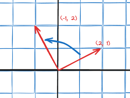
Let’s try to get some intuition for some of the linear transformation. For example if we have vector \(\begin{bmatrix} 2 \\ 1 \end{bmatrix}\), how can we rotate it 90 degrees counter-clockwise?
We can do that by visualizing how he vector end up after the transformation. For our matrix of \(\begin{bmatrix} 2 \\ 1 \end{bmatrix}\), we can see that after the transformation, the vector end up at \(\begin{bmatrix} -1 \\ 2 \end{bmatrix}\).
So how do we deduce the transformation matrix from that?
As we can see, our previous \(\begin{bmatrix} x \\ y \end{bmatrix}\) is transformed to \(\begin{bmatrix} -y \\ x \end{bmatrix}\). And because transformation matrix rows and columns must match the dimension of the vector that we’re transforming, we can define below matrix
\[ \begin{bmatrix} a & b \\ c & d \end{bmatrix} \begin{bmatrix} x \\ y \end{bmatrix} = \begin{bmatrix} -y \\ x \end{bmatrix} \]
\(a\) can be thought as what value from previous x that we want to put to the new \(x\), let’s say it’s \(x'\).
\[ \begin{bmatrix} a & b \\ c & d \end{bmatrix} \begin{bmatrix} x \\ y \end{bmatrix} = \begin{bmatrix} -y \\ x \end{bmatrix} = \begin{bmatrix} x' \\ y' \end{bmatrix} \]
Which as we can see that
\[ ax + by = -y = x' \\ cx + dy = x = y' \]
As we can see from our transformed matrix which is \(\begin{bmatrix} -y \\ x \end{bmatrix}\), the previous \(x\) is not carried over to \(x'\) (because as we can see that \(x'\) = \(-y\)), so we can deduce that \(a\) is 0.
\[ 0x + by = -y = x' \\ by = -y \\ b = -1 \]
Next for \(cx + dy = x = y'\), we can deduce that \(y\) is not carried over to \(y'\) because \(y'\) = \(x\), so we can deduce that \(d\) is 0.
\[ cx + 0y = x = y' \\ cx = x \\ c = 1 \]
So now we can deduce that our transformation matrix for 90 degrees counter-clockwise rotation is
\[ \begin{bmatrix} 0 & -1 \\ 1 & 0 \end{bmatrix} \]
Exercise 1
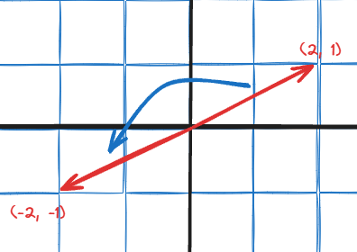
Above is a visualization of a linear transformation of 180 degrees rotation. Try to deduce the transformation matrix for this linear transformation.
Note: The submission will be in python list such as
[[a, b], [c, d]], where it will be equivalent to \(\begin{bmatrix} a & b \\ c & d \end{bmatrix}\) matrix
from rggrader import submit

# @title #### Student Identity
student_id = "your student id" # @param {type:"string"}
name = "your name" # @param {type:"string"}
assignment_id = "14_linear-algebra"
question_id = "01_180_rotation_matrix"
matrix = [[0, 0], [0, 0]]
submit(student_id, name, assignment_id, str(matrix), question_id)Exercise 2
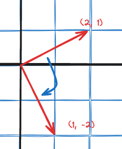
Above is the visualization of a linear transformation of 90 degrees clockwise rotation. Try to deduce the transformation matrix for this linear transformation.
!pip install rggraderfrom rggrader import submit
# @title #### Student Identity
student_id = "your student id" # @param {type:"string"}
name = "your name" # @param {type:"string"}assignment_id = "14_linear-algebra"
question_id = "02_90_rotation_matrix"
matrix = [[0, 0], [0, 0]]
submit(student_id, name, assignment_id, str(matrix), question_id)Vectors vs Points
In linear algebra, we’re working with vectors, but we can use points to represent vectors visually especially if we’re working with lots of vectors - It’s just get overwhelming to see bunch of arrows rather than just bunch of dots.
There should be a video above, if it does not load, click this link: Multiple Data Matrix Multiplication With Points
Vector length
The length of a vector is the distance from the origin of the dimensional space to the vector’s position. The length of a vector is also known as the magnitude of a vector.
Norm
Manhattan norm
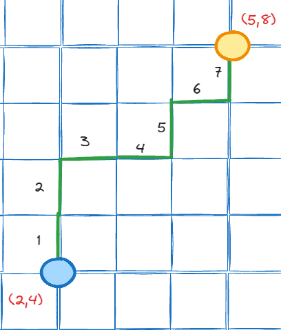
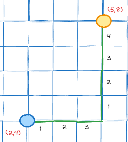
Manhattan norm is how to measure distance between 2 points by “walking” through the grid without ever going diagonally. So for above 2 vectors we have (2, 4) and (5, 8), and by counting every step we take to reach the destination, we can calculate the distance between those 2 vectors is 7.
Now, let’s generalize. Above steps that we’ve taken basically can be rearranged to below image
And above image can be summarized to below image
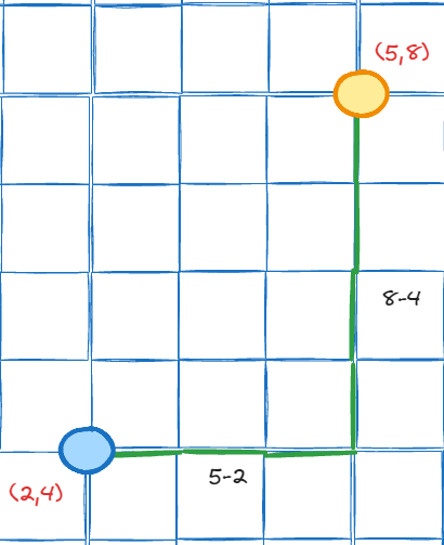
So basically on manhattan norm we can calculate the distance from (2, 4) to (5, 8) by walking 3 steps to the right (5 is our destination, and 2 is our origin, 5 - 2 = 3) and 4 steps to the top (8 is our destination, and 4 is our origin, 8 - 4 = 4). So the distance is 3 + 4 = 7. If we formalize it, we have below formula:
\[ \text{Manhattan norm} = |a_1 - b_1| + |a_2 - b_2| \]
Where a is our origin and b is our destination and the subscript 1 and 2 is the single data point on that vector (eg \(a_1\) is the first data point on vector a, for vector of (2, 4) it will be 2, and for vector of (5, 8) it will be 5).
This can later be generalized to more than 2 dimensions:
\[ \text{Manhattan norm} = \sum_{i=1}^{n} |a_i - b_i| \]
Where n is the number of dimensions/features of the vector.
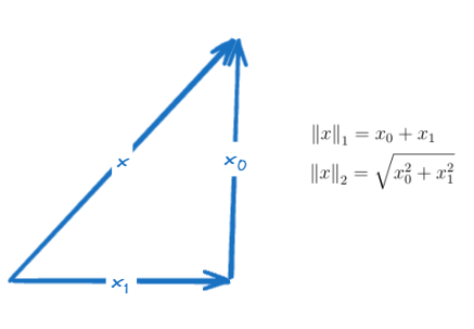
Note that the notation for the manhattan norm is \(||x||_1\) or \(||x||_M\)
Euclidean norm
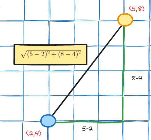
After understanding manhattan norm, euclidean norm can be understood easily. Euclidean norm is basically “enabling” us to go diagonally. So for above 2 vectors we have (2, 4) and (5, 8), and by using pythagoras theorem we can calculate the distance between those 2 vectors is
\[ \sqrt{(5 - 2)^2 + (8 - 4)^2} = \sqrt{9 + 16} = \sqrt{25} = 5 \]
This pythagoras theorem can held true for any number of dimensions, so we can generalize it to below formula:
\[ \text{Euclidean norm} = \sqrt{\sum_{i=1}^{n} (a_i - b_i)^2} \]
Where n is the number of dimensions/features of the vector.
Then the notation for the euclidean norm is \(||x||_2\), and most of the times if no subscript is given (only \(||x||\)), it most likely means euclidean norm.
Summarization of manhattan and euclidean norm
To summarize between manhattan and euclidean norm, below is the visualization:
Hundreds Of Dimensions And the Amazing Applications
Linear algebra allowing us to “playing” with higher-dimensional space, so the calculation is not bound to 2 or 3 dimensions. We can have hundreds of dimensions, even thousands of dimensions, even though it’s impossible for us to visualize it, because we can just scale the calculation that we have on 2 and 3 dimensions to higher dimensions. For our learning we’ll mostly working with 2 dimensions to make it easier to visualize and understand, but every formula is scalable to billions of dimensions.
This kind of calculation is basically what is happening in Natural Language Processing (NLP), Computer Vision (CV), Audio Processing, and other fields that are using deep learning. The data is mostly saved as a matrix with hundreds or thousands of dimensions, and then it’s processed by calculating it with other matrices, and then the result is converted back to something that we as humans can understand. Amazing isn’t it? A really complex machine learning models like GPT is basically just a bunch of matrix multiplications, data transformed in higher dimensional space, and then converted back to something that we can understand, by, again, just a bunch of matrix multiplications.