Deep Learning Model

Deep Learning consists of neural networks with many layers. The layers are connected to each other and each layer has a weight. The weight is used to calculate the output of each layer. The output of the previous layer is used as the input of the next layer. The output of the last layer is the output of the model.

So what is neural networks?

Neural Networks

Neural Networks consists of neurons. Each neuron has inputs, weights, bias, an activation function, and an output.

from fastbook import *


# Draw neurons with multiple inputs and weights
gv('''
z[shape=box3d width=1 height=0.7]
bias[shape=circle width=0.3]
// Subgraph to force alignment on x-axis
subgraph {
    rank=same;
    z;
    bias;
    alignmentNode [style=invis, width=0]; // invisible node for alignment
    bias -> alignmentNode [style=invis]; // invisible edge
    z -> alignmentNode [style=invis]; // invisible edge
}
x_0->z [label="w_0"]
x_1->z [label="w_1"]
bias->z [label="b" pos="0,1.2!"]
z->output [label="z = w_0 x_0 + w_1 x_1 + b"]
''')

We can have multiple neurons in one layer

from fastbook import *

# Draw neurons with multiple inputs and weights
gv('''
z0[shape=box3d width=1 height=0.7]
z1[shape=box3d width=1 height=0.7]
bias_0[shape=circle width=0.3]
bias_1[shape=circle width=0.3]

subgraph {
    rank=same;
    z0;
    bias_0;
    alignmentNode [style=invis, width=0]; // invisible node for alignment
    bias_0 -> alignmentNode [style=invis]; // invisible edge
    z0 -> alignmentNode [style=invis]; // invisible edge
}

subgraph {
    rank=same;
    z1;
    bias_1;
    alignmentNode [style=invis, width=0]; // invisible node for alignment
    bias_1 -> alignmentNode [style=invis]; // invisible edge
    z1 -> alignmentNode [style=invis]; // invisible edge
}
x_0->z0 [label="w_0,0"]
x_1->z0 [label="w_0,1"]
bias_0->z0 [label="b_0" pos="0,1.2!"]
z0->output_0 [label="z0 = w_0,0 x_0 + w_0,1 x_1 + b_0"]
   
x_0->z1 [label="w_1,0"]
x_1->z1 [label="w_1,1"]
bias_1->z1 [label="b_1" pos="0,1.2!"]
z1->output_1 [label="z1 = w_1,0 x_0 + w_1,1 x_1 + b_1"]
''')

Multilayer Neural Networks

The output of the previous layer can be used as the input of the next layer. The output of the last layer is the output of the model.

from fastbook import *

gv('''
   x_0 -> z_0_0
   x_0 -> z_0_1
   x_1 -> z_0_0
   x_1 -> z_0_1
   z_0_0 -> z_1_0
   z_0_1 -> z_1_0
   z_1_0 -> output
   ''')

Note that the network is fully connected, so the following is not a valid network

from fastbook import *

gv('''
   x_0 -> z_0_0
   x_1 -> z_0_1
   z_0_0 -> z_1_0
   z_0_1 -> z_1_0
   z_1_0 -> output
   ''')

Vectorized

Operations in neurons can be vectorized. This is important because it can speed up the calculation.

It also simplifies the code. Let’s go back to the previous example.

from fastbook import *


# Draw neurons with multiple inputs and weights
gv('''
z[shape=box3d width=1 height=0.7]
bias[shape=circle width=0.3]
// Subgraph to force alignment on x-axis
subgraph {
    rank=same;
    z;
    bias;
    alignmentNode [style=invis, width=0]; // invisible node for alignment
    bias -> alignmentNode [style=invis]; // invisible edge
    z -> alignmentNode [style=invis]; // invisible edge
}
x_0->z [label="w_0"]
x_1->z [label="w_1"]
bias->z [label="b" pos="0,1.2!"]
z->output [label="z = w_0 x_0 + w_1 x_1 + b"]
''')

Matrix representation

\[ x = \begin{bmatrix} x_0 \\ x_1 \end{bmatrix} \]

\[ w = \begin{bmatrix} w_0 & w_1 \end{bmatrix} \]

\[ b = \begin{bmatrix} b_0 \end{bmatrix} \]

\[ z = wx + b \]

If we have multiple neurons in one layer, we can write it as follow

from fastbook import *

# Draw neurons with multiple inputs and weights
gv('''
z0[shape=box3d width=1 height=0.7]
z1[shape=box3d width=1 height=0.7]
bias_0[shape=circle width=0.3]
bias_1[shape=circle width=0.3]

subgraph {
    rank=same;
    z0;
    bias_0;
    alignmentNode [style=invis, width=0]; // invisible node for alignment
    bias_0 -> alignmentNode [style=invis]; // invisible edge
    z0 -> alignmentNode [style=invis]; // invisible edge
}

subgraph {
    rank=same;
    z1;
    bias_1;
    alignmentNode [style=invis, width=0]; // invisible node for alignment
    bias_1 -> alignmentNode [style=invis]; // invisible edge
    z1 -> alignmentNode [style=invis]; // invisible edge
}
x_0->z0 [label="w_0,0"]
x_1->z0 [label="w_0,1"]
bias_0->z0 [label="b_0" pos="0,1.2!"]
z0->output_0 [label="z0 = w_0,0 x_0 + w_0,1 x_1 + b_0"]
   
x_0->z1 [label="w_1,0"]
x_1->z1 [label="w_1,1"]
bias_1->z1 [label="b_1" pos="0,1.2!"]
z1->output_1 [label="z1 = w_1,0 x_0 + w_1,1 x_1 + b_1"]
''')

Matrix representation

\[ x = \begin{bmatrix} x_0 \\ x_1 \end{bmatrix} \]

\[ w = \begin{bmatrix} w_{00} & w_{01} \\ w_{10} & w_{11} \end{bmatrix} \]

\[ b = \begin{bmatrix} b_0 \\ b_1 \end{bmatrix} \]

\[ z = wx + b \]

Let’s try 3 neurons and 2 inputs

from fastbook import *

gv('''
   x_0 -> z_0
   x_0 -> z_1
   x_0 -> z_2
   x_1 -> z_0
   x_1 -> z_1
   x_1 -> z_2
   z_0 -> output_0
   z_1 -> output_1
   z_2 -> output_2
   ''')

Matrix representation

\[ x = \begin{bmatrix} x_0 \\ x_1 \end{bmatrix} \]

\[ w = \begin{bmatrix} w_{00} & w_{01} \\ w_{10} & w_{11} \\ w_{20} & w_{21} \end{bmatrix} \]

\[ b = \begin{bmatrix} b_0 \\ b_1 \\ b_2 \end{bmatrix} \]

\[ z = wx + b \]

Lastly, let’s try vectorized multi layers

from fastbook import *

gv('''
   x_0 -> z_0_0
   x_0 -> z_0_1
   x_1 -> z_0_0
   x_1 -> z_0_1
   z_0_0 -> z_1_0
   z_0_1 -> z_1_0
   z_1_0 -> output
   ''')

Matrix representation

\[ x = \begin{bmatrix} x_0 \\ x_1 \end{bmatrix} \]

First layer

\[ w^{[0]} = \begin{bmatrix} w_{00} & w_{01} \\ w_{10} & w_{11} \\ \end{bmatrix} \]

\[ b^{[0]} = \begin{bmatrix} b_0 \\ b_1 \end{bmatrix} \]

\[ z^{[0]} = w^{[0]}x + b^{[0]} \]

Second layer

\[ w^{[1]} = \begin{bmatrix} w_{00} & w_{01} \end{bmatrix} \]

\[ b^{[1]} = \begin{bmatrix} b_0 \end{bmatrix} \]

\[ z^{[1]} = w^{[1]}z^{[0]} + b^{[1]} \]

We can write the full equation as follow

\[ z^{[1]} = w^{[1]}(w^{[0]}x + b^{[0]}) + b^{[1]} = w^{[1]}w^{[0]}x + w^{[1]}b^{[0]} + b^{[1]} \]

Activation Function

Notice the equation above:

\[ z^{[1]} = w^{[1]}w^{[0]}x + w^{[1]}b^{[0]} + b^{[1]} \]

By associativity, we can write it as follow

\[ z^{[1]} = (w^{[1]}w^{[0]})x + w^{[1]}b^{[0]} + b^{[1]} \]

Let’s substitute \[ W = w^{[1]}w^{[0]} \]

\[ z^{[1]} = Wx + (w^{[1]}b^{[0]} + b^{[1]}) = Wx + B \]

The final equation is still linear, it doesn’t differ from a single layer.

By being linear the final equation would still be a straight line.

To introduce non-linearity, we need to add an activation function.

\[ a^{[0]} = g(z^{[0]}) \]

from fastbook import *


# Draw neurons with multiple inputs and weights
gv('''
z[shape=box3d width=1 height=0.7]
bias[shape=circle width=0.3]
// Subgraph to force alignment on x-axis
subgraph {
    rank=same;
    z;
    bias;
    alignmentNode [style=invis, width=0]; // invisible node for alignment
    bias -> alignmentNode [style=invis]; // invisible edge
    z -> alignmentNode [style=invis]; // invisible edge
}
x_0->z [label="w_0"]
x_1->z [label="w_1"]
bias->z [label="b" pos="0,1.2!"]
z->a [label="z = w_0 x_0 + w_1 x_1 + b"]
a->output [label="a = g(z)"]
''')

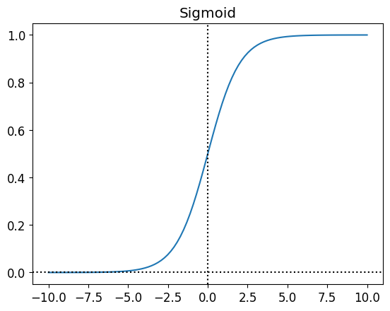
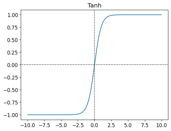
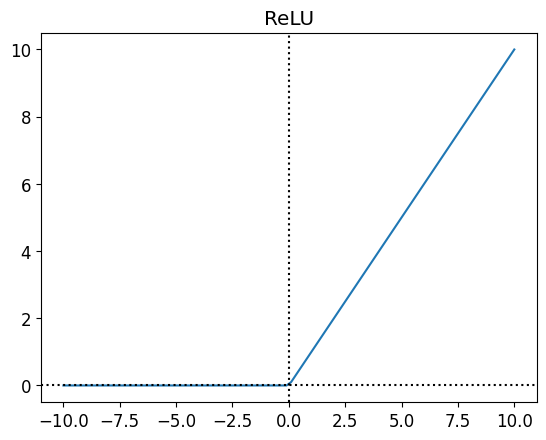
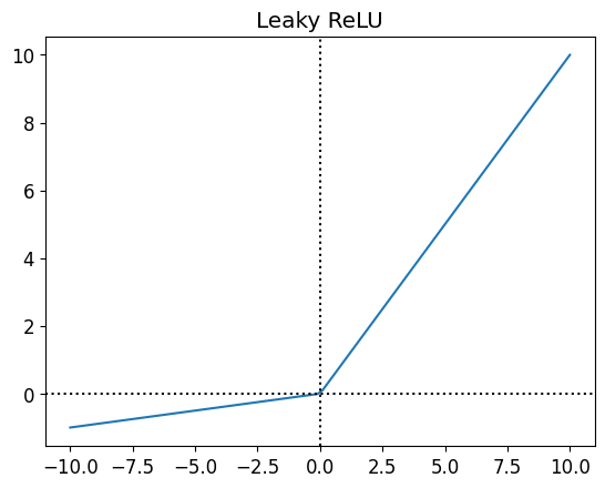
There are many activation functions, but the most common ones are: - Sigmoid \[ g(z) = \frac{1}{1 + e^{-z}} \] - Tanh \[ g(z) = \frac{e^z - e^{-z}}{e^z + e^{-z}} \] - ReLU \[ g(z) = max(0, z) \] - Leaky ReLU \[ g(z) = max(0.01z, z) \]

The decision to use which activation function depends on the problem. - Sigmoid used to be the most popular activation function, but it has a problem called vanishing gradient. It means that the gradient becomes very small and the model doesn’t learn anymore. - Tanh is similar to sigmoid, but it has a range from -1 to 1. - ReLU is the most popular activation function right now. It is simple and it doesn’t have vanishing gradient problem. - Leaky ReLU is a variation of ReLU. It is used to solve the dying ReLU problem. Dying ReLU is a problem where the neuron doesn’t activate anymore because the input is always negative.

# Draw sigmoid, tanh, ReLU, and Leaky ReLU activation functions using matplotlib

import matplotlib.pyplot as plt
import numpy as np

x = np.linspace(-10, 10, 100)
sigmoid = 1/(1+np.exp(-x))
tanh = (np.exp(x)-np.exp(-x))/(np.exp(x)+np.exp(-x))
relu = np.maximum(0, x)
leaky_relu = np.maximum(0.1*x, x)

# Draw each in a separate plot
plt.plot(x, sigmoid)
plt.title("Sigmoid")
# Draw x and y axes, make it dotted
plt.axhline(y=0, color='k', linestyle='dotted')
plt.axvline(x=0, color='k', linestyle='dotted')
plt.show()

plt.plot(x, tanh)
plt.title("Tanh")
plt.axhline(y=0, color='k', linestyle='dotted')
plt.axvline(x=0, color='k', linestyle='dotted')
plt.show()

plt.plot(x, relu)
plt.title("ReLU")
plt.axhline(y=0, color='k', linestyle='dotted')
plt.axvline(x=0, color='k', linestyle='dotted')
plt.show()

plt.plot(x, leaky_relu)
plt.title("Leaky ReLU")
plt.axhline(y=0, color='k', linestyle='dotted')
plt.axvline(x=0, color='k', linestyle='dotted')
plt.show()

Matrix Representation with Activation Function

Let’s try to add activation function to the previous example

\[ x = \begin{bmatrix} x_0 \\ x_1 \end{bmatrix} \]

First layer

\[ w^{[0]} = \begin{bmatrix} w_{00} & w_{01} \\ w_{10} & w_{11} \\ \end{bmatrix} \]

\[ b^{[0]} = \begin{bmatrix} b_0 \\ b_1 \end{bmatrix} \]

\[ z^{[0]} = w^{[0]}x + b^{[0]} \]

\[ a^{[0]} = g^{[0]}(z^{[0]}) \]

Second layer

\[ w^{[1]} = \begin{bmatrix} w_{00} & w_{01} \end{bmatrix} \]

\[ b^{[1]} = \begin{bmatrix} b_0 \end{bmatrix} \]

\[ z^{[1]} = w^{[1]}a^{[0]} + b^{[1]} \]

\[ a^{[1]} = g^{[1]}(z^{[1]}) \]

We can write the full equation as follow

\[ a^{[1]} = g^{[1]}(w^{[1]}(g^{[0]}(w^{[0]}x + b^{[0]})) + b^{[1]}) \]

Let’s wrap up with a diagram of multi layer NN with activation functions

from fastbook import *

gv('''
   x_0 -> z_0_0 
   x_0 -> z_0_1 
   x_1 -> z_0_0
   x_1 -> z_0_1
   z_0_0 -> a_0_0 -> z_1_0
   z_0_1 -> a_0_1 -> z_1_0
   z_1_0 -> a_1_0 -> output
   ''')

Cost Function

The cost function formula for multi layer NN is the same as the single layer NN:

\[ J = \frac{1}{m}\sum_{i=1}^{m}L(\hat{y}^{(i)}, y^{(i)}) \]

or can also be simplified as

\[ J = \sum_{i=1}^{m}L(a^{[L](i)}, y^{(i)}) \]