Today we will learn about calculus, which is the study of change. Calculus is a branch of mathematics that is used to study continuous change. It has two main branches: differential calculus and integral calculus. Differential calculus is used to study the rate of change of a function, while integral calculus is used to study the accumulation of quantities, or the area under a curve.
Derivatives
We all - probably know - that the derivative of
\[
f(x) = 2x^3 + 3x^2 + 2x + 5
\]
is \[
f'(x) = 6x^2 + 6x + 2
\]
But what does that mean?
The derivative of a function \(f(x)\) is actually defined as:
\[
\frac{df(x)}{dx} = \lim_{\delta \to 0} \frac{f(x+\delta) - f(x)}{\delta}
\]
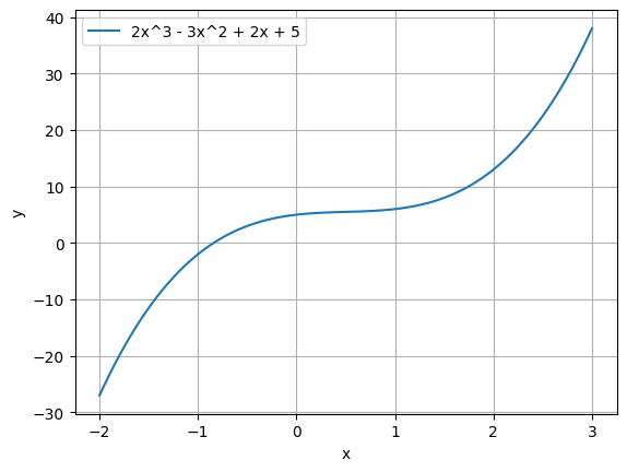
To understand what this means, let’s plot \(f(x)\) and \(f'(x)\) .
# Plot 2x^3 - 3x^2 + 2x + 5 import numpy as npimport matplotlib.pyplot as plt= np.linspace(- 2 , 3 , 100 )= 2 * x** 3 - 3 * x** 2 + 2 * x + 5 'x' )'y' )# add legend '2x^3 - 3x^2 + 2x + 5' ])
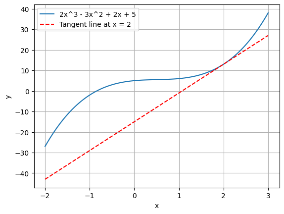
Now, let’s plot a tangent line to \(f(x)\) at \(x=2\) .
# Plot 2x^3 - 3x^2 + 2x + 5 import numpy as npimport matplotlib.pyplot as plt= np.linspace(- 2 , 3 , 100 )= 2 * x** 3 - 3 * x** 2 + 2 * x + 5 # Tangent line at x = 2 = 2 = 2 * x1** 3 - 3 * x1** 2 + 2 * x1 + 5 = 6 * x1** 2 - 6 * x1 + 2 = m* (x - x1) + y1# Plot the main function # Plot tangent line 'r--' )'2x^3 - 3x^2 + 2x + 5' , 'Tangent line at x = 2' ])'x' )'y' )
What is the slope of the tangent line at \(x=2\) ?
That’s right, it’s \(f'(2)\) .
But - without the knowledge of calculus - how would we calculate that slope?
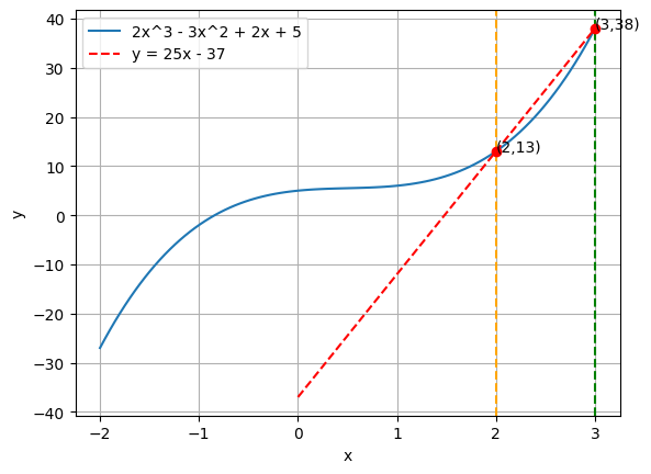
Actually we can, we just need to zoom in and calculate the slope of the line that is “close enough” to the tangent line.
# Plot 2x^3 - 3x^2 + 2x + 5 import numpy as npimport matplotlib.pyplot as pltdef f(x):return 2 * x** 3 - 3 * x** 2 + 2 * x + 5 = np.linspace(- 2 , 3 , 100 )= f(x)# Plot the main function # Create a vertical line at x = 2 and x = 3 = 2 , color= 'orange' , linestyle= '--' )= 3 , color= 'g' , linestyle= '--' )'2x^3 - 3x^2 + 2x + 5' ])= 2 = f(x1)# create a dot at (x1, y1) with label (2, y1) 'ro' )'( {} , {} )' .format (x1, y1), xy= (x1, y1), xytext= (x1, y1))= 3 = f(x2)# create a dot at (x2, y2) with label (3, y2) 'ro' )'( {} , {} )' .format (x2, y2), xy= (x2, y2), xytext= (x2, y2))'x' )'y' )
Then create a straight line from \(x=2\) to \(x=3\) .
The slope of that line is:
\[
m = \frac{f(3) - f(2)}{3 - 2}
= \frac{38-13}{3-2}
= 25
\]
The y-intercept of that line is:
\[
f(x) = mx + c\\
c = f(x) - mx
\]
Substitute \(x=2\) and \(y=f(2)\) : \[
c = f(2) - m \cdot 2
= 13 - 25 \cdot 2
= -37
\]
So the equation of the line is: \[
y = 25x - 37
\]
Let’s draw that line.
# Plot 2x^3 - 3x^2 + 2x + 5 import numpy as npimport matplotlib.pyplot as pltdef f(x):return 2 * x** 3 - 3 * x** 2 + 2 * x + 5 = np.linspace(- 2 , 3 , 100 )= f(x)# Plot the main function = '2x^3 - 3x^2 + 2x + 5' )# Create a vertical line at x = 2 and x = 3 = 2 , color= 'orange' , linestyle= '--' )= 3 , color= 'g' , linestyle= '--' )= 2 = f(x1)# create a dot at (x1, y1) with label (2, y1) 'ro' )'( {} , {} )' .format (x1, y1), xy= (x1, y1), xytext= (x1, y1))= 3 = f(x2)# create a dot at (x2, y2) with label (3, y2) 'ro' )'( {} , {} )' .format (x2, y2), xy= (x2, y2), xytext= (x2, y2))# Draw y = 25x - 37 = np.linspace(0 , 3 , 100 )= 25 * x3 - 37 'r--' , label= 'y = 25x - 37' )'x' )'y' )
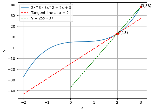
Now we know that the slop is \(37\) , but that’s not the exact slope of the tangent line.
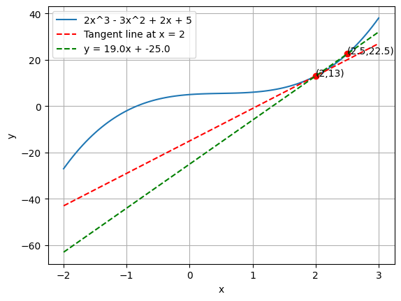
Let’s draw both lines together
# Plot 2x^3 - 3x^2 + 2x + 5 import numpy as npimport matplotlib.pyplot as plt= np.linspace(- 2 , 3 , 100 )= 2 * x** 3 - 3 * x** 2 + 2 * x + 5 # Tangent line at x = 2 = 2 = 2 * x1** 3 - 3 * x1** 2 + 2 * x1 + 5 = 6 * x1** 2 - 6 * x1 + 2 = m* (x - x1) + y1# Plot the main function = "2x^3 - 3x^2 + 2x + 5" )# Plot tangent line 'r--' , label= 'Tangent line at x = 2' )= 2 = f(x1)# create a dot at (x1, y1) with label (2, y1) 'ro' )'( {} , {} )' .format (x1, y1), xy= (x1, y1), xytext= (x1, y1))= 3 = f(x2)# create a dot at (x2, y2) with label (3, y2) 'ro' )'( {} , {} )' .format (x2, y2), xy= (x2, y2), xytext= (x2, y2))# Draw y = 25x - 37 = np.linspace(0 , 3 , 100 )= 25 * x3 - 37 'g--' , label= 'y = 25x - 37' )'x' )'y' )
Hmm, not quite right. Perhaps, let’s try drawing line at x = 2$ and \(x = 2.5\) ?
# Plot 2x^3 - 3x^2 + 2x + 5 import numpy as npimport matplotlib.pyplot as plt= np.linspace(- 2 , 3 , 100 )= 2 * x** 3 - 3 * x** 2 + 2 * x + 5 # Tangent line at x = 2 = 2 = 2 * x1** 3 - 3 * x1** 2 + 2 * x1 + 5 = 6 * x1** 2 - 6 * x1 + 2 = m* (x - x1) + y1# Plot the main function = "2x^3 - 3x^2 + 2x + 5" )# Plot tangent line 'r--' , label= 'Tangent line at x = 2' )= 2 = f(x1)# create a dot at (x1, y1) with label (2, y1) 'ro' )'( {} , {} )' .format (x1, y1), xy= (x1, y1), xytext= (x1, y1))= 2.5 = f(x2)# create a dot at (x2, y2) with label (3, y2) 'ro' )'( {} , {} )' .format (x2, y2), xy= (x2, y2), xytext= (x2, y2))= (y2 - y1) / (x2 - x1)= y2 - m* x2= m* x + c'g--' , label= 'y = {} x + {} ' .format (m, c))'x' )'y' )
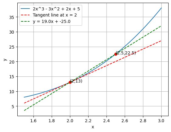
It’s getting closer to the tangent line. Let’s zoom in the graph
# Plot 2x^3 - 3x^2 + 2x + 5 import numpy as npimport matplotlib.pyplot as plt= np.linspace(1.5 , 3 , 100 )= 2 * x** 3 - 3 * x** 2 + 2 * x + 5 # Tangent line at x = 2 = 2 = 2 * x1** 3 - 3 * x1** 2 + 2 * x1 + 5 = 6 * x1** 2 - 6 * x1 + 2 = m* (x - x1) + y1# Plot the main function = "2x^3 - 3x^2 + 2x + 5" )# Plot tangent line 'r--' , label= 'Tangent line at x = 2' )= 2 = f(x1)# create a dot at (x1, y1) with label (2, y1) 'ro' )'( {} , {} )' .format (x1, y1), xy= (x1, y1), xytext= (x1, y1))= 2.5 = f(x2)# create a dot at (x2, y2) with label (3, y2) 'ro' )'( {} , {} )' .format (x2, y2), xy= (x2, y2), xytext= (x2, y2))= (y2 - y1) / (x2 - x1)= y2 - m* x2= m* x + c'g--' , label= 'y = {} x + {} ' .format (m, c))'x' )'y' )
The idea is, if we can get \(x_2\) closer to \(x_1\) , we can get the slope of the line closer to the tangent line.
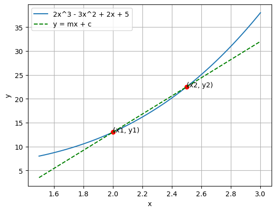
Let’s try to generalize
# Plot 2x^3 - 3x^2 + 2x + 5 import numpy as npimport matplotlib.pyplot as plt= np.linspace(1.5 , 3 , 100 )= 2 * x** 3 - 3 * x** 2 + 2 * x + 5 # Plot the main function = "2x^3 - 3x^2 + 2x + 5" )= 2 = f(x1)# create a dot at (x1, y1) with label (2, y1) 'ro' )'(x1, y1)' , xy= (x1, y1), xytext= (x1, y1))= 2.5 = f(x2)# create a dot at (x2, y2) with label (3, y2) 'ro' )'(x2, y2)' , xy= (x2, y2), xytext= (x2, y2))= (y2 - y1) / (x2 - x1)= y2 - m* x2= m* x + c'g--' , label= 'y = mx + c' )'x' )'y' )
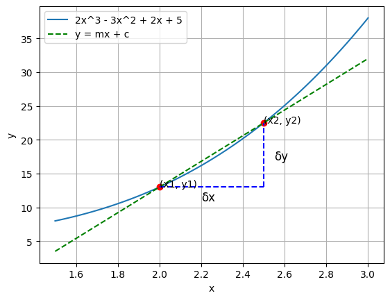
To find the slope, we need to find the change in \(y\) divided by the change in \(x\) .
# Plot 2x^3 - 3x^2 + 2x + 5 import numpy as npimport matplotlib.pyplot as plt= np.linspace(1.5 , 3 , 100 )= 2 * x** 3 - 3 * x** 2 + 2 * x + 5 # Plot the main function = "2x^3 - 3x^2 + 2x + 5" )= 2 = f(x1)# create a dot at (x1, y1) with label (2, y1) 'ro' )'(x1, y1)' , xy= (x1, y1), xytext= (x1, y1))= 2.5 = f(x2)# create a dot at (x2, y2) with label (3, y2) 'ro' )'(x2, y2)' , xy= (x2, y2), xytext= (x2, y2))= (y2 - y1) / (x2 - x1)= y2 - m* x2= m* x + c'g--' , label= 'y = mx + c' )= np.linspace(x1, x2, 100 )= np.linspace(y1, y1, 100 )'b--' )# add text near that plot 2.2 , 11 , 'δx' , fontsize= 12 )= np.linspace(x2, x2, 100 )= np.linspace(y1, y2, 100 )'b--' )# add text near that plot 2.55 , 17 , 'δy' , fontsize= 12 )'x' )'y' )
The slope \(m\) is:
\[
m = \frac{f(x_2) - f(x_1)}{x_2 - x_1}
\]
\[
m = \frac{f(x_1 + \delta x) - f(x_1)}{\delta x}
\]
Since \(m\) is \(\frac{\delta y}{\delta x}\)
\[
\frac{\delta y}{\delta x} = \frac{f(x_1 + \delta x) - f(x_1)}{\delta x}
\]
If we let \(\delta x\) approach \(0\) , we get the tangent line:
\[
\frac{df(x)}{dx} = \lim_{\delta x \to 0} \frac{f(x_1 + \delta x) - f(x_1)}{\delta x}
\]
Interestingly, we can derive many different derivative formula using this method.
For example, the derivative of \(f(x) = x^2\) is:
\[
\frac{df(x)}{dx} = \lim_{\delta x \to 0} \frac{(x + \delta x)^2 - x^2}{\delta x}
= \lim_{\delta x \to 0} \frac{x^2 + 2x\delta x + \delta x^2 - x^2}{\delta x}
= \lim_{\delta x \to 0} \frac{2x\delta x + \delta x^2}{\delta x}
= \lim_{\delta x \to 0} 2x + \delta x
\]
Since \(\delta x\) approaches \(0\) , we can ignore it:
\[
\frac{df(x)}{dx} = 2x
\]
One more example, the derivative of \(f(x) = x^3\) is:
\[
\frac{df(x)}{dx} = \lim_{\delta x \to 0} \frac{(x + \delta x)^3 - x^3}{\delta x}
= \lim_{\delta x \to 0} \frac{x^3 + 3x^2\delta x + 3x\delta x^2 + \delta x^3 - x^3}{\delta x}
= \lim_{\delta x \to 0} \frac{3x^2\delta x + 3x\delta x^2 + \delta x^3}{\delta x}
= \lim_{\delta x \to 0} 3x^2 + 3x\delta x + \delta x^2
\]
Since \(\delta x\) approaches \(0\) , we can ignore it:
\[
\frac{df(x)}{dx} = 3x^2
\]
Derivative rules
Here we only list down the rules, but actually the concepts are simple.
Please watch the following videos:
Visualizing the chain rule and product rule | Chapter 4, Essence of calculus
Addition rule
\[
\frac{d}{dx} (f(x) + g(x)) = \frac{df(x)}{dx} + \frac{dg(x)}{dx}
\]
Example:
\[
\frac{d}{dx} (x^2 + 2x) = \frac{d}{dx} (x^2) + \frac{d}{dx} (2x) = 2x + 2
\]
Multiplication rule
\[
\frac{d}{dx} (f(x) \cdot g(x)) = f(x) \cdot \frac{dg(x)}{dx} + g(x) \cdot \frac{df(x)}{dx}
\]
Example:
\[
\frac{d}{dx} (x^2 \cdot 2x) = x^2 \cdot \frac{d}{dx} (2x) + 2x \cdot \frac{d}{dx} (x^2) = x^2 \cdot 2 + 2x \cdot 2x = 6x^2
\]
Power rule
\[
\frac{d}{dx} (x^n) = n \cdot x^{n-1}
\]
Example:
\[
\frac{d}{dx} (x^3) = 3x^2
\]
Chain rule
\[
\frac{d}{dx} f(g(x)) = \frac{df(g(x))}{dg(x)} \cdot \frac{dg(x)}{dx}
\]
Or it can also be written as:
Let’s denote \(u = g(x)\) :
\[
\frac{d}{dx} f(u) = \frac{df(u)}{du} \cdot \frac{du}{dx}
\]
Please remember this rule, it will be used a lot in deep learning.