Gradient Descent with PyTorch

import torch

x = torch.tensor(5, requires_grad=True, dtype=torch.float32)
# quadratic function
y = x**2 + 2*x + 1

# plot the function from x = 0 to x = 10
import matplotlib.pyplot as plt
import numpy as np
x_plt = np.linspace(-10, 10, 100)
y_plt = x_plt**2 + 2*x_plt + 1
plt.plot(x_plt, y_plt)
plt.title('y = x^2 + 2x + 1')

# Plot the x, y
plt.plot(x.detach().numpy(), y.detach().numpy(), 'o')
plt.show()

What is the gradient at x = 5?

In the previous notebook, we have learned the hardway:

• Calculate the derivative of a function
• Apply the derivative to \(x\) to find the gradient at \(x\)

But in PyTorch, we can do it in a much easier way.

from fastbook import *

gv('''
   x -> y[label="x^2 + 2x+1"]
   ''')

x = torch.tensor(5, requires_grad=True, dtype=torch.float32)
y = x**2 + 2*x + 1

# compute gradient
y.backward()

# print gradient
print(x.grad)

tensor(12.)

backward() does backward propagation to calculate the gradient. And the result is stored in x.grad.

Notice the requires_grad=True in the definition of x. It tells PyTorch to calculate the gradient of x during backward propagation. If we don’t set it, x.grad will raise an error.

x = torch.tensor(5, requires_grad=False, dtype=torch.float32)
y = x**2 + 2*x + 1

# compute gradient
y.backward()

# Error
print(x.grad)

Let’s find the minimum value like before. Remember the steps:

1. Initialize \(x\) at a random value
2. Calculate the gradient at \(x\)
3. Update \(x\) with the gradient with a learning rate \(\alpha\) (\(x = x - \alpha \cdot \text{gradient}\))
4. Repeat 2 and 3 until the gradient is close to 0

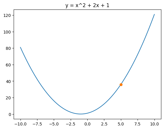
# Randomly choose x
x = torch.tensor(5, requires_grad=True, dtype=torch.float32)
alpha = 0.1

for i in range(10):
    y = x**2 + 2*x + 1
    y.backward()
    
    with torch.no_grad():
        x -= alpha * x.grad
        # gradient is accumulated, so we need to zero it
        x.grad.zero_()

    print(x.detach().numpy(), y.detach().numpy())
    

3.8 36.0
2.84 23.039999
2.072 14.7456
1.4576 9.437184
0.96607995 6.039798
0.57286394 3.8654704
0.25829116 2.473901
0.006632924 1.5832967
-0.19469367 1.0133098
-0.35575494 0.6485183

Let’s visualize the process.

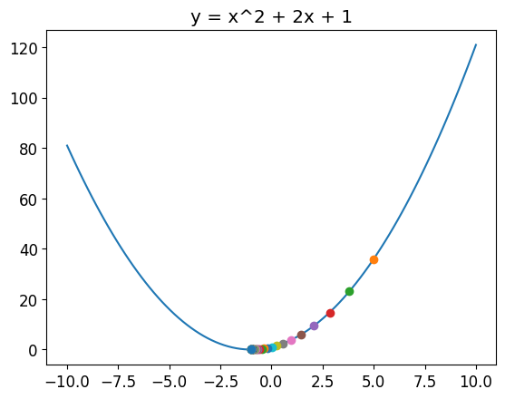
# Randomly choose x
x = torch.tensor(5, requires_grad=True, dtype=torch.float32)
alpha = 0.1

x_plt = np.linspace(-10, 10, 100)
y_plt = x_plt**2 + 2*x_plt + 1
plt.plot(x_plt, y_plt)
plt.title('y = x^2 + 2x + 1')

# Plot the 
for i in range(50):
    y = x**2 + 2*x + 1
    plt.plot(x.detach().numpy(), y.detach().numpy(), 'o')

    y.backward()

    gradient = None
    with torch.no_grad():
        gradient = x.grad.item()
        x -= alpha * x.grad
        # gradient is accumulated, so we need to zero it
        x.grad.zero_()

    print(x.detach().numpy(), y.detach().numpy(), gradient)

plt.show()

3.8 36.0 12.0
2.84 23.039999 9.600000381469727
2.072 14.7456 7.679999828338623
1.4576 9.437184 6.144000053405762
0.96607995 6.039798 4.915200233459473
0.57286394 3.8654704 3.932159900665283
0.25829116 2.473901 3.1457278728485107
0.006632924 1.5832967 2.5165822505950928
-0.19469367 1.0133098 2.01326584815979
-0.35575494 0.6485183 1.6106126308441162
-0.48460394 0.4150517 1.2884900569915771
-0.58768314 0.2656331 1.0307921171188354
-0.6701465 0.1700052 0.8246337175369263
-0.73611724 0.10880327 0.6597069501876831
-0.7888938 0.06963408 0.5277655124664307
-0.83111507 0.044565797 0.4222123622894287
-0.86489207 0.028522134 0.33776986598968506
-0.89191365 0.01825416 0.27021586894989014
-0.91353095 0.01168263 0.2161726951599121
-0.93082476 0.007476926 0.17293810844421387
-0.9446598 0.0047852397 0.1383504867553711
-0.9557279 0.0030625463 0.11068034172058105
-0.9645823 0.0019600391 0.08854424953460693
-0.97166586 0.0012544394 0.07083535194396973
-0.9773327 0.00080281496 0.05666828155517578
-0.9818662 0.00051379204 0.045334577560424805
-0.98549294 0.00032883883 0.036267638206481934
-0.9883944 0.000210464 0.029014110565185547
-0.9907155 0.0001347065 0.023211240768432617
-0.9925724 8.6188316e-05 0.018568992614746094
-0.99405795 5.51939e-05 0.014855146408081055
-0.99524635 3.528595e-05 0.011884093284606934
-0.9961971 2.259016e-05 0.009507298469543457
-0.99695766 1.4483929e-05 0.007605791091918945
-0.9975661 9.23872e-06 0.0060846805572509766
-0.9980529 5.90086e-06 0.0048677921295166016
-0.9984423 3.8146973e-06 0.003894209861755371
-0.99875385 2.4437904e-06 0.003115415573120117
-0.99900305 1.5497208e-06 0.0024923086166381836
-0.99920243 1.013279e-06 0.001993894577026367
-0.99936193 6.556511e-07 0.001595139503479004
-0.99948955 4.172325e-07 0.0012761354446411133
-0.99959165 2.3841858e-07 0.0010209083557128906
-0.9996733 1.7881393e-07 0.0008167028427124023
-0.99973863 1.1920929e-07 0.000653386116027832
-0.9997909 5.9604645e-08 0.0005227327346801758
-0.99983275 5.9604645e-08 0.0004181861877441406
-0.9998662 0.0 0.0003345012664794922
-0.99989295 0.0 0.0002676248550415039
-0.99991435 0.0 0.00021409988403320312

Optimizer

In the previous example, we have to manually update \(x\) with the gradient. But in PyTorch, we can use an optimizer to do it for us.

torch.optim.SGD is a simple optimizer that does gradient descent. It takes the parameters to optimize and the learning rate as arguments.

# Randomly choose x
x = torch.tensor(5, requires_grad=True, dtype=torch.float32)
alpha = 0.1
optimizer = torch.optim.SGD([x], lr=alpha)

for i in range(10):
    y = x**2 + 2*x + 1
    y.backward()
    
    optimizer.step()
    optimizer.zero_grad()

    print(x.detach().numpy(), y.detach().numpy())
    

3.8 36.0
2.84 23.039999
2.072 14.7456
1.4576 9.437184
0.96607995 6.039798
0.57286394 3.8654704
0.25829116 2.473901
0.006632924 1.5832967
-0.19469367 1.0133098
-0.35575494 0.6485183

We get the same result as before, but with less code (without manually updating \(x\)).

There are some other optimizers, such as torch.optim.Adam and torch.optim.RMSprop. You can find more in the documentation.

Building Simple Neural Networks

We now know how to calculate the gradient of a function and use an optimizer to find the minimum value. We can use this knowledge to build a simple neural network.

Let’s build NOT gate with a single neuron, similar to what we have here

x = torch.tensor([[0], [1]], dtype=torch.float32)
y = torch.tensor([1, 0], dtype=torch.float32)

w = torch.tensor([[3]], requires_grad=True, dtype=torch.float32)
b = torch.tensor([[1]], requires_grad=True, dtype=torch.float32)

a = torch.sigmoid(w@x.T + b)

print("a = ", a)

loss = torch.square(a - y)
print("loss = ", loss.detach().numpy())

loss = torch.mean(loss)
print("sum loss = ", loss.detach().numpy())

loss.backward()

print("w_grad = ", w.grad)
print("b_grad = ", b.grad)

a =  tensor([[0.7311, 0.9820]], grad_fn=<SigmoidBackward0>)
loss =  [[0.07232948 0.96435106]]
sum loss =  0.5183403
w_grad =  tensor([[0.0173]])
b_grad =  tensor([[-0.0355]])

That’s similar to what we got in the Google Sheet. Do check it out if you haven’t :)

Now, we just need to iterate.

import torch

x = torch.tensor([[0], [1]], dtype=torch.float32)
y = torch.tensor([1, 0], dtype=torch.float32)

w = torch.tensor([[3]], requires_grad=True, dtype=torch.float32)
b = torch.tensor([[1]], requires_grad=True, dtype=torch.float32)

optimizer = torch.optim.SGD([w, b], lr=10)

for i in range(5):
    print("Iteration ", i)
    print("w = ", w.detach().numpy())
    print("b = ", b.detach().numpy())

    a = torch.sigmoid(w@x.T + b)

    print("a = ", a)

    loss = torch.square(a - y)
    print("loss = ", loss.detach().numpy())

    loss = torch.mean(loss)
    print("mean loss = ", loss.detach().numpy())

    loss.backward()

    print("w_grad = ", w.grad)
    print("b_grad = ", b.grad)

    # Update w, b
    optimizer.step()
    optimizer.zero_grad()
    
    print()

Iteration  0
w =  [[3.]]
b =  [[1.]]
a =  tensor([[0.7311, 0.9820]], grad_fn=<SigmoidBackward0>)
loss =  [[0.07232948 0.96435106]]
mean loss =  0.5183403
w_grad =  tensor([[0.0173]])
b_grad =  tensor([[-0.0355]])

Iteration  1
w =  [[2.8265495]]
b =  [[1.3553205]]
a =  tensor([[0.7950, 0.9850]], grad_fn=<SigmoidBackward0>)
loss =  [[0.0420258  0.97014576]]
mean loss =  0.50608575
w_grad =  tensor([[0.0146]])
b_grad =  tensor([[-0.0188]])

Iteration  2
w =  [[2.6806374]]
b =  [[1.5435127]]
a =  tensor([[0.8240, 0.9856]], grad_fn=<SigmoidBackward0>)
loss =  [[0.03098487 0.97135484]]
mean loss =  0.50116986
w_grad =  tensor([[0.0140]])
b_grad =  tensor([[-0.0115]])

Iteration  3
w =  [[2.5405035]]
b =  [[1.6586863]]
a =  tensor([[0.8401, 0.9852]], grad_fn=<SigmoidBackward0>)
loss =  [[0.02558029 0.970647  ]]
mean loss =  0.49811363
w_grad =  tensor([[0.0144]])
b_grad =  tensor([[-0.0071]])

Iteration  4
w =  [[2.3969853]]
b =  [[1.7300583]]
a =  tensor([[0.8494, 0.9841]], grad_fn=<SigmoidBackward0>)
loss =  [[0.02267439 0.96850324]]
mean loss =  0.4955888
w_grad =  tensor([[0.0154]])
b_grad =  tensor([[-0.0039]])

Compare it with the Google Sheet. It’s the same!

Simpler Way to Build Neural Networks

Our code looks much simpler than before. But we can make it even simpler with torch.nn.

import torch

x = torch.tensor([[0], [1]], dtype=torch.float32)
y = torch.tensor([1, 0], dtype=torch.float32)

class NotGate(torch.nn.Module):
    def __init__(self):
        super().__init__()
        self.w = torch.nn.Parameter(torch.tensor([[3.]]))
        self.b = torch.nn.Parameter(torch.tensor([[1.]]))
    
    def forward(self, x):
        return torch.sigmoid(self.w@x.T + self.b)

model = NotGate()
optimizer = torch.optim.SGD(model.parameters(), lr=10)

for i in range(5):
    print("Iteration ", i)
    print("w = ", model.w.detach().numpy())
    print("b = ", model.b.detach().numpy())

    model.train()
    a = model(x)

    print("a = ", a)

    loss = torch.square(a - y)
    print("loss = ", loss.detach().numpy())

    loss = torch.mean(loss)
    print("mean loss = ", loss.detach().numpy())

    loss.backward()

    print("w_grad = ", model.w.grad)
    print("b_grad = ", model.b.grad)

    # Update w, b
    optimizer.step()
    optimizer.zero_grad()
    
    print()

Iteration  0
w =  [[3.]]
b =  [[1.]]
a =  tensor([[0.7311, 0.9820]], grad_fn=<SigmoidBackward0>)
loss =  [[0.07232948 0.96435106]]
mean loss =  0.5183403
w_grad =  tensor([[0.0173]])
b_grad =  tensor([[-0.0355]])

Iteration  1
w =  [[2.8265495]]
b =  [[1.3553205]]
a =  tensor([[0.7950, 0.9850]], grad_fn=<SigmoidBackward0>)
loss =  [[0.0420258  0.97014576]]
mean loss =  0.50608575
w_grad =  tensor([[0.0146]])
b_grad =  tensor([[-0.0188]])

Iteration  2
w =  [[2.6806374]]
b =  [[1.5435127]]
a =  tensor([[0.8240, 0.9856]], grad_fn=<SigmoidBackward0>)
loss =  [[0.03098487 0.97135484]]
mean loss =  0.50116986
w_grad =  tensor([[0.0140]])
b_grad =  tensor([[-0.0115]])

Iteration  3
w =  [[2.5405035]]
b =  [[1.6586863]]
a =  tensor([[0.8401, 0.9852]], grad_fn=<SigmoidBackward0>)
loss =  [[0.02558029 0.970647  ]]
mean loss =  0.49811363
w_grad =  tensor([[0.0144]])
b_grad =  tensor([[-0.0071]])

Iteration  4
w =  [[2.3969853]]
b =  [[1.7300583]]
a =  tensor([[0.8494, 0.9841]], grad_fn=<SigmoidBackward0>)
loss =  [[0.02267439 0.96850324]]
mean loss =  0.4955888
w_grad =  tensor([[0.0154]])
b_grad =  tensor([[-0.0039]])

Even Much More Simpler Way

We can make it even simpler with torch.nn.Linear.

from fastbook import *

gv('''
x -> NotGate -> y
''')

import torch

x = torch.tensor([[0], [1]], dtype=torch.float32)
y = torch.tensor([1, 0], dtype=torch.float32)

class NotGate(torch.nn.Module):
    def __init__(self):
        super().__init__()
        self.linear = torch.nn.Linear(in_features=1, out_features=1)
    
    def forward(self, x):
        return torch.sigmoid(self.linear(x))
    
model = NotGate()
optimizer = torch.optim.SGD(model.parameters(), lr=10)

for i in range(5):
    print("Iteration ", i)
    print("w = ", model.linear.weight.detach().numpy())
    print("b = ", model.linear.bias.detach().numpy())

    model.train()
    a = model(x)

    print("a = ", a)

    loss = torch.square(a - y)
    print("loss = ", loss.detach().numpy())

    loss = torch.mean(loss)
    print("mean loss = ", loss.detach().numpy())

    loss.backward()

    print("w_grad = ", model.linear.weight.grad)
    print("b_grad = ", model.linear.bias.grad)

    # Update w, b
    optimizer.step()
    optimizer.zero_grad()
    
    print()

Iteration  0
w =  [[-0.08132863]]
b =  [0.9673029]
a =  tensor([[0.7246],
        [0.7081]], grad_fn=<SigmoidBackward0>)
loss =  [[0.07585529 0.5250185 ]
 [0.08522972 0.5013471 ]]
mean loss =  0.29686266
w_grad =  tensor([[0.0430]])
b_grad =  tensor([0.0878])

Iteration  1
w =  [[-0.5114101]]
b =  [0.0890395]
a =  tensor([[0.5222],
        [0.3959]], grad_fn=<SigmoidBackward0>)
loss =  [[0.22824968 0.27274   ]
 [0.3648769  0.15677612]]
mean loss =  0.25566065
w_grad =  tensor([[-0.0249]])
b_grad =  tensor([-0.0193])

Iteration  2
w =  [[-0.26254913]]
b =  [0.28239763]
a =  tensor([[0.5701],
        [0.5050]], grad_fn=<SigmoidBackward0>)
loss =  [[0.18478484 0.32505268]
 [0.24506265 0.25498658]]
mean loss =  0.2524717
w_grad =  tensor([[0.0012]])
b_grad =  tensor([0.0184])

Iteration  3
w =  [[-0.27495283]]
b =  [0.09810886]
a =  tensor([[0.5245],
        [0.4559]], grad_fn=<SigmoidBackward0>)
loss =  [[0.22609304 0.27510822]
 [0.29604056 0.20784836]]
mean loss =  0.25127253
w_grad =  tensor([[-0.0109]])
b_grad =  tensor([-0.0048])

Iteration  4
w =  [[-0.16556998]]
b =  [0.14636995]
a =  tensor([[0.5365],
        [0.4952]], grad_fn=<SigmoidBackward0>)
loss =  [[0.21480696 0.28786153]
 [0.25482288 0.24522316]]
mean loss =  0.25067863
w_grad =  tensor([[-0.0012]])
b_grad =  tensor([0.0079])

Here we just need to define the input size and output size. We don’t need to define the weights and bias manually!

from fastbook import *

gv('''
   x_0[label=3]
   x_1[label=5]
   a_0_0[label="b=8, ReLU"]
   a_0_1[label="b=-2, ReLU"]
   a_0_2[label="b=4, ReLU"]
   a_1_0[label="b=3, ReLU"]
   x_0 -> a_0_0 [label=-2]
   x_0 -> a_0_1 [label=5]
   x_0 -> a_0_2 [label=3]
   x_1 -> a_0_0 [label=8]
   x_1 -> a_0_1 [label=-2]
   x_1 -> a_0_2 [label=4]
   a_0_0 -> a_1_0 [label=3]
   a_0_1 -> a_1_0 [label=2]
   a_0_2 -> a_1_0 [label=8]
   
   a_1_0 -> output
   ''')

class ComplexNetwork(torch.nn.Module):
    def __init__(self):
        super().__init__()
        self.linear1 = torch.nn.Linear(in_features=2, out_features=3)
        self.linear2 = torch.nn.Linear(in_features=3, out_features=1)
    
    def forward(self, x):
        x = torch.relu(self.linear1(x))
        x = torch.relu(self.linear2(x))
        return x

model = ComplexNetwork()
optimizer = torch.optim.SGD(model.parameters(), lr=0.1)

x = torch.tensor([[3, 5]], dtype=torch.float32)
y = torch.tensor([[10]], dtype=torch.float32)

for i in range(5):
    model.train()
    y_hat = model(x)

    loss = torch.square(y_hat - y)
    loss = torch.mean(loss)

    loss.backward()

    optimizer.step()
    optimizer.zero_grad()

    print("Iteration ", i)
    print("w1 = ", model.linear1.weight.detach().numpy())
    print("b1 = ", model.linear1.bias.detach().numpy())
    print("w2 = ", model.linear2.weight.detach().numpy())
    print("b2 = ", model.linear2.bias.detach().numpy())

    print("loss = ", loss.detach().numpy())

Iteration  0
w1 =  [[-1.3071573  -1.9972436 ]
 [ 2.1915283   4.3640413 ]
 [ 0.10451669 -0.33010566]]
b1 =  [-0.28740007  0.43799853 -0.08292443]
w2 =  [[ 4.097638    4.571283   -0.45574307]]
b2 =  [1.728075]
loss =  99.424774
Iteration  1
w1 =  [[-1.30715728e+00 -1.99724364e+00]
 [-3.36625305e+02 -5.60330750e+02]
 [ 1.04516685e-01 -3.30105662e-01]]
b1 =  [-2.87400067e-01 -1.12500946e+02 -8.29244256e-02]
w2 =  [[ 4.0976381e+00 -7.0777679e+02 -4.5574307e-01]]
b2 =  [-22.978106]
loss =  15259.883
Iteration  2
w1 =  [[-1.30715728e+00 -1.99724364e+00]
 [-3.36625305e+02 -5.60330750e+02]
 [ 1.04516685e-01 -3.30105662e-01]]
b1 =  [-2.87400067e-01 -1.12500946e+02 -8.29244256e-02]
w2 =  [[ 4.0976381e+00 -7.0777679e+02 -4.5574307e-01]]
b2 =  [-22.978106]
loss =  100.0
Iteration  3
w1 =  [[-1.30715728e+00 -1.99724364e+00]
 [-3.36625305e+02 -5.60330750e+02]
 [ 1.04516685e-01 -3.30105662e-01]]
b1 =  [-2.87400067e-01 -1.12500946e+02 -8.29244256e-02]
w2 =  [[ 4.0976381e+00 -7.0777679e+02 -4.5574307e-01]]
b2 =  [-22.978106]
loss =  100.0
Iteration  4
w1 =  [[-1.30715728e+00 -1.99724364e+00]
 [-3.36625305e+02 -5.60330750e+02]
 [ 1.04516685e-01 -3.30105662e-01]]
b1 =  [-2.87400067e-01 -1.12500946e+02 -8.29244256e-02]
w2 =  [[ 4.0976381e+00 -7.0777679e+02 -4.5574307e-01]]
b2 =  [-22.978106]
loss =  100.0